Cited by 127

The DOI matches its Crossref record; 2 of the 2 references it cites were found in a registry or an index.

Mapped aboveground carbon stocks to advance forest conservation and recovery in Malaysian Borneo

Asner, Gregory P., Brodrick, Philip G., Philipson, Christopher, Vaughn, Nicolas R., Martin, Roberta E., Knapp, David E., Heckler, Joseph, Evans, Luke J., Jucker, Tommaso, Goossens, Benoit, Stark, Danica J., Reynolds, Glen, Ong, Robert, Renneboog, Nathan, Kugan, Fred, Coomes, David A.·2018·Biological Conservation

Overview

The claims and statistics of this paper haven’t been checked yet.

Run the check — free, no account needed. It reads the open-access text and checks the sources it cites.

A few free checks a day · papers already verified open instantly · results are public

Integrity signals

Registry

Crossref · 10.1016/j.biocon.2017.10.020

Cites

2 of 2 references verified0 citation errors · 0 not checkable

Statistics

Figures

Image 1
CC-BY · From the PDF
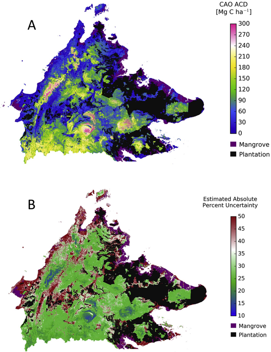
Fig. 1 (A) Aboveground carbon density (ACD) throughout the State of Sabah in Malaysian Borneo, at 30 m (0.09 ha) spatial resolution. Areas covered by mangrove and oil palm plantation are masked out. (B) Estimated absolute uncertainty in units of percent of mapped ACD at 30 m (0.09 ha) resolution.
Fig. 1 (A) Aboveground carbon density (ACD) throughout the State of Sabah in Malaysian Borneo, at 30 m (0.09 ha) spatial resolution. Areas covered by mangrove and oil palm plantation are masked out. (B) Estimated absolute uncertainty in units of percent of mapped ACD at 30 m (0.09 ha) resolution.CC-BY · From the PDF
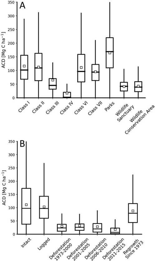
Fig. 2 (A) Aboveground carbon density (ACD) statistics throughout the State of Sabah sorted by forest management class (see Fig. A1). (B) ACD statistics by land cover classifi cation of Gaveau et al. (2016). Red dots and lines are mean and median ACD values. Box plots indicate one standard deviation, and whiskers indicate data range.
Fig. 2 (A) Aboveground carbon density (ACD) statistics throughout the State of Sabah sorted by forest management class (see Fig. A1). (B) ACD statistics by land cover classifi cation of Gaveau et al. (2016). Red dots and lines are mean and median ACD values. Box plots indicate one standard deviation, and whiskers indicate data range.CC-BY · From the PDF
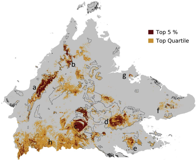
Fig. 3 Locations of the top 5% and top quartile of aboveground carbon densities (ACD) for natural forests of Sabah, Malaysia, not including mangroves. Thin black lines indicate the location of Sabah Forest ' Class I ' and ' Parks ' designated reserves, which are the most protected in the State. Lettering highlights areas of high carbon stock forest including (a) Crocker Range, (b) Mount Kinabalu area, (c) Maliau Basin and Imbak Canyon, (d) Danum Valley, (e) Tawau Hills area, (f) Tabin area, (g) Sepilok, and (h) southwestern Sabah near to the Sarawak, Malaysia and Kalimantan, Indonesian borders.
Fig. 3 Locations of the top 5% and top quartile of aboveground carbon densities (ACD) for natural forests of Sabah, Malaysia, not including mangroves. Thin black lines indicate the location of Sabah Forest ' Class I ' and ' Parks ' designated reserves, which are the most protected in the State. Lettering highlights areas of high carbon stock forest including (a) Crocker Range, (b) Mount Kinabalu area, (c) Maliau Basin and Imbak Canyon, (d) Danum Valley, (e) Tawau Hills area, (f) Tabin area, (g) Sepilok, and (h) southwestern Sabah near to the Sarawak, Malaysia and Kalimantan, Indonesian borders.CC-BY · From the PDF
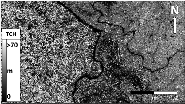
Fig. 4 Forest top-of-canopy height (TCH) where unlogged forest (left side of river) abuts a previously logged forest within Danum Valley, Sabah, Malaysia.
Fig. 4 Forest top-of-canopy height (TCH) where unlogged forest (left side of river) abuts a previously logged forest within Danum Valley, Sabah, Malaysia.CC-BY · From the PDF
Image 6
CC-BY · From the PDF
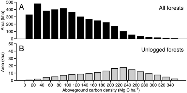
Fig. 5 (A) Distribution of aboveground carbon density (ACD) for natural forests throughout Sabah. (B) Distribution for unlogged natural forests only.
Fig. 5 (A) Distribution of aboveground carbon density (ACD) for natural forests throughout Sabah. (B) Distribution for unlogged natural forests only.CC-BY · From the PDF
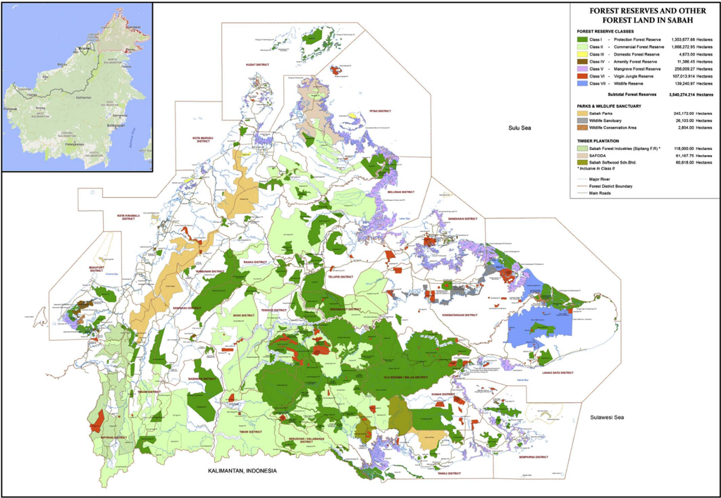
Fig. A1. Statewide distribution of o ffi cial forest reserves and other forest lands throughout Sabah, Malaysia. Map courtesy of Sabah Forestry Department. Inset map shows the location of Sabah outlined in red on the island of Borneo.
Fig. A1. Statewide distribution of o ffi cial forest reserves and other forest lands throughout Sabah, Malaysia. Map courtesy of Sabah Forestry Department. Inset map shows the location of Sabah outlined in red on the island of Borneo.CC-BY · From the PDF
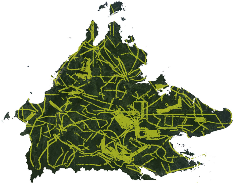
Fig. A2. Distribution of data collection fl ightlines from the Carnegie Airborne Observatory sampling of Sabah. Each line is 1.5 -3.0 km wide (swath). Areas of particularly concentrated mapping coincide with landscapes containing fi eld calibration plots.
Fig. A2. Distribution of data collection fl ightlines from the Carnegie Airborne Observatory sampling of Sabah. Each line is 1.5 -3.0 km wide (swath). Areas of particularly concentrated mapping coincide with landscapes containing fi eld calibration plots.CC-BY · From the PDF
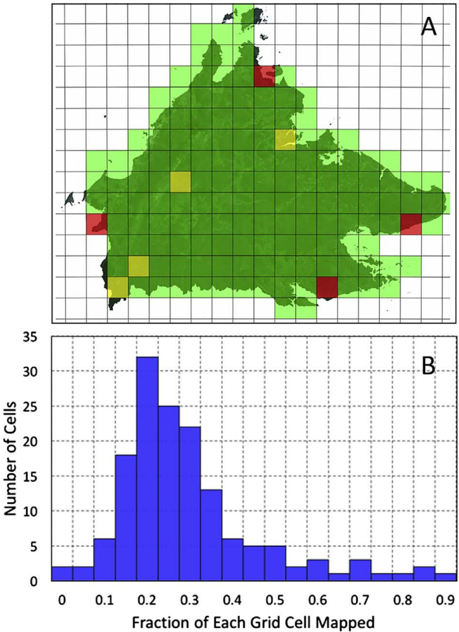
Fig. A3. (A) Resulting of near real-time modeling of Carnegie Airborne Observatory data density required to fully meet data sampling requirements. Green indicates 100% coverage, yellow indicates 95% coverage, and red indicates 90% coverage. Grid lines indicate mapping units of 25 km × 25 km. (B) The fraction each 25 km × 25 km grid cell mapping unit covered during CAO data collection fl ights. (For interpretation of the references to colour in this fi gure legend, the reader is referred to the web version of this article.)
Fig. A3. (A) Resulting of near real-time modeling of Carnegie Airborne Observatory data density required to fully meet data sampling requirements. Green indicates 100% coverage, yellow indicates 95% coverage, and red indicates 90% coverage. Grid lines indicate mapping units of 25 km × 25 km. (B) The fraction each 25 km × 25 km grid cell mapping unit covered during CAO data collection fl ights. (For interpretation of the references to colour in this fi gure legend, the reader is referred to the web version of this article.)CC-BY · From the PDF
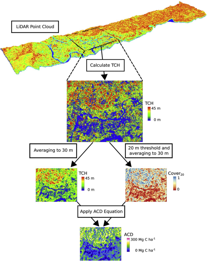
Fig. A4. Work fl ow illustrating how airborne LiDAR point cloud data are used to estimate aboveground carbon density (ACD). First, tree canopy height (TCH) is calculated from the point cloud at 2 m ground-level resolution. Next, TCH is averaged to 30 m resolution, and the fraction of 2 m TCH pixels that exceed 20 m is used to determine Cover20 at 30 m resolution. Finally, we calculate aboveground carbon density (ACD) as a function of TCH and Cover20 (see main text).
Fig. A4. Work fl ow illustrating how airborne LiDAR point cloud data are used to estimate aboveground carbon density (ACD). First, tree canopy height (TCH) is calculated from the point cloud at 2 m ground-level resolution. Next, TCH is averaged to 30 m resolution, and the fraction of 2 m TCH pixels that exceed 20 m is used to determine Cover20 at 30 m resolution. Finally, we calculate aboveground carbon density (ACD) as a function of TCH and Cover20 (see main text).CC-BY · From the PDF
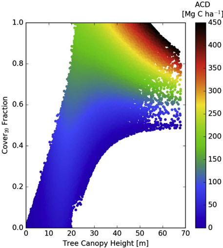
Fig. A5. Aboveground carbon density (ACD) as a function of top-of-canopy height (TCH) and the fraction of the canopy that exceeds 20 m (Cover20) for all CAO fl ight data (see main text for equation).
Fig. A5. Aboveground carbon density (ACD) as a function of top-of-canopy height (TCH) and the fraction of the canopy that exceeds 20 m (Cover20) for all CAO fl ight data (see main text for equation).CC-BY · From the PDF
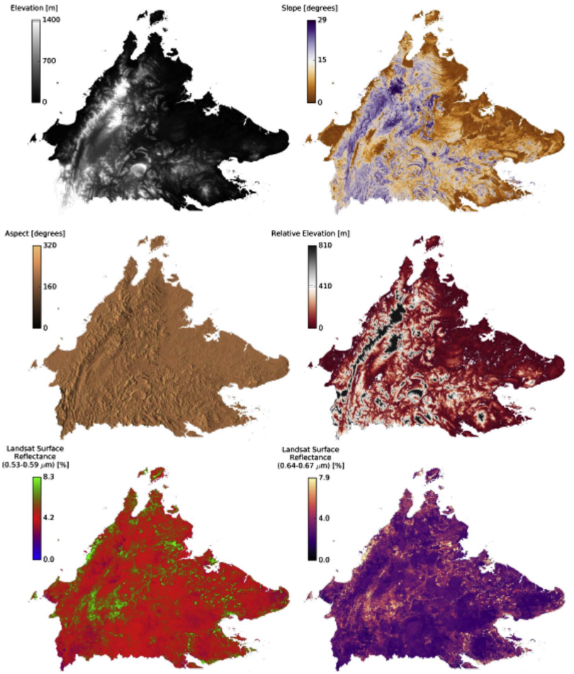
Fig. A6. Six of the environmental dataset layers used in upscaling airborne LiDAR to the Sabah level. Topographic elevation, slope, aspect, and relative elevation were derived from NASA SRTM data, and Landsat-8 surface re fl ectance data were composited between 15 Oct 2015 and 15 Oct 2016 to generate a cloud-free mosaic.
Fig. A6. Six of the environmental dataset layers used in upscaling airborne LiDAR to the Sabah level. Topographic elevation, slope, aspect, and relative elevation were derived from NASA SRTM data, and Landsat-8 surface re fl ectance data were composited between 15 Oct 2015 and 15 Oct 2016 to generate a cloud-free mosaic.CC-BY · From the PDF
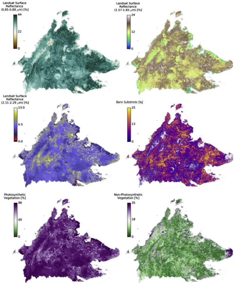
Fig. A7. Six of the environmental dataset layers used in upscaling airborne LiDAR to the Sabah level. Landsat-8 surface re fl ectance data were composited between 15 Oct 2015 and 15 Oct 2016 to generate a cloud-free mosaic. Bare substrate, photosynthetic, and non-photosynthetic vegetation were derived from Landsat-8 surface re fl ectance data.
Fig. A7. Six of the environmental dataset layers used in upscaling airborne LiDAR to the Sabah level. Landsat-8 surface re fl ectance data were composited between 15 Oct 2015 and 15 Oct 2016 to generate a cloud-free mosaic. Bare substrate, photosynthetic, and non-photosynthetic vegetation were derived from Landsat-8 surface re fl ectance data.CC-BY · From the PDF
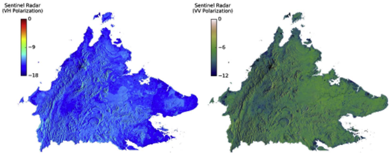
Fig. A8. Two of the environmental dataset layers used in upscaling airborne LiDAR to the Sabah level. Sentinel synthetic aperture radar (SAR) data with VH and VV polarizations were collected using the interferometric wide swath mode were aggregated between 1 Feb 2016 and 1 July 2016 using the per-pixel median to account for view-angle e ff ects.
Fig. A8. Two of the environmental dataset layers used in upscaling airborne LiDAR to the Sabah level. Sentinel synthetic aperture radar (SAR) data with VH and VV polarizations were collected using the interferometric wide swath mode were aggregated between 1 Feb 2016 and 1 July 2016 using the per-pixel median to account for view-angle e ff ects.CC-BY · From the PDF
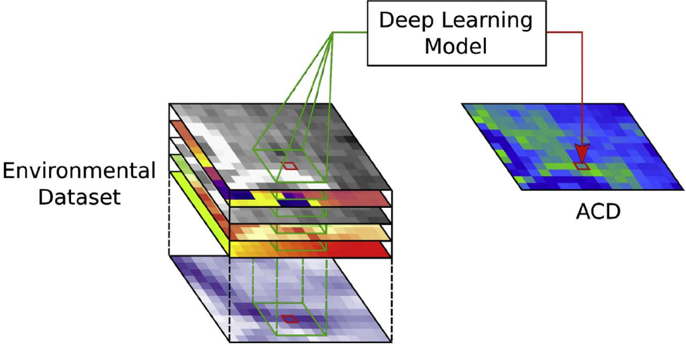
Fig. A9. Visualization of the deep learning model-based upscaling process. Data from each layer in the environmental dataset in a 5 × 5 pixel window (shown in green) around the target pixel (shown in red) are used in each model prediction. (For interpretation of the references to colour in this fi gure legend, the reader is referred to the web version of this article.)
Fig. A9. Visualization of the deep learning model-based upscaling process. Data from each layer in the environmental dataset in a 5 × 5 pixel window (shown in green) around the target pixel (shown in red) are used in each model prediction. (For interpretation of the references to colour in this fi gure legend, the reader is referred to the web version of this article.)CC-BY · From the PDF
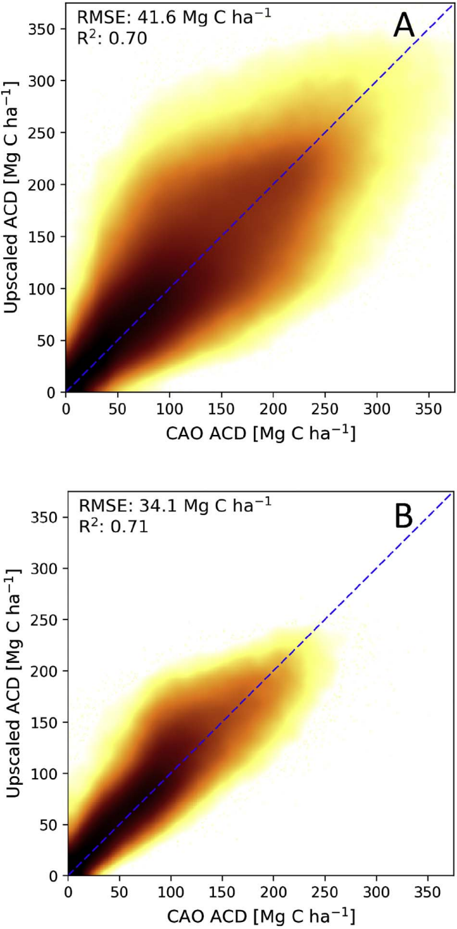
Fig. A10. Veri fi cation that ACD estimated from airborne LiDAR data are represented in the upscaled Sabah-wide ACD map. The deviation is shown for both the (A) 30 m resolution data and (B) one-hectare resolution. Both plots show minimal bias, and the hectare average shows reduced variation compared with the 30 m resolution predictions.
Fig. A10. Veri fi cation that ACD estimated from airborne LiDAR data are represented in the upscaled Sabah-wide ACD map. The deviation is shown for both the (A) 30 m resolution data and (B) one-hectare resolution. Both plots show minimal bias, and the hectare average shows reduced variation compared with the 30 m resolution predictions.CC-BY · From the PDF
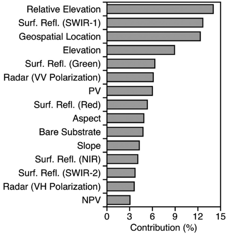
Fig. A11. The in fl uence of each mapped environmental factor (Figs. A6 -A8) on upscaling model performance. In order of contribution, the features are relative elevation, Landsat-8 surface re fl ectance (Surf. Re fl .) from the SWIR-1 band, geospatial location, elevation, Landsat-8 surface re fl ectance from the green band, radar data in the VV polarization, photosynthetic vegetation (PV), Landsat-8 surface re fl ectance from the red band, aspect, bare substrate, slope, Landsat-8 surface re fl ectance from the NIR band, Landsat-8 surface re fl ectance from the SWIR-2 band, radar data in the VH polarization, and non-photosynthetic vegetation (NPV). (For interpretation of the references to colour in this fi gure legend, the reader is referred to the web version of this article.)
Fig. A11. The in fl uence of each mapped environmental factor (Figs. A6 -A8) on upscaling model performance. In order of contribution, the features are relative elevation, Landsat-8 surface re fl ectance (Surf. Re fl .) from the SWIR-1 band, geospatial location, elevation, Landsat-8 surface re fl ectance from the green band, radar data in the VV polarization, photosynthetic vegetation (PV), Landsat-8 surface re fl ectance from the red band, aspect, bare substrate, slope, Landsat-8 surface re fl ectance from the NIR band, Landsat-8 surface re fl ectance from the SWIR-2 band, radar data in the VH polarization, and non-photosynthetic vegetation (NPV). (For interpretation of the references to colour in this fi gure legend, the reader is referred to the web version of this article.)CC-BY · From the PDF

Verification

Claims the paper makes

The claims and statistics of this paper haven’t been checked yet.

Run the check — free, no account needed. It reads the open-access text and checks the sources it cites.

A few free checks a day · papers already verified open instantly · results are public

Claims other papers make about this one

Each is checked against this paper’s own text: does it say what the citing paper says it does?

Self-check

Percentages, sums and reported differences re-computed from the paper’s own numbers.

The self-check needs the paper’s full text.

Citations

Cites

Research works printed but not linked: 34

  1. Ashton, 1992, Comparisons of structure among mixed dipterocarp forests of north-western Borneo, J. Ecol., 459, 10.2307/2260691 · DOI
  2. Asner, 2014, Mapping tropical forest carbon: calibrating plot estimates to a simple LiDAR metric, Remote Sens. Environ., 140, 614, 10.1016/j.rse.2013.09.023 · DOI
  3. Asner, 2009, Automated mapping of tropical deforestation and forest degradation: CLASlite, J. Appl. Remote. Sens., 3, 10.1117/1.3223675 · DOI
  4. Asner, 2012, Human and environmental controls over aboveground carbon storage in Madagascar, Carbon Balance Manag., 7, 2, 10.1186/1750-0680-7-2 · DOI
  5. Asner, 2012, Carnegie airborne observatory-2: increasing science data dimensionality via high-fidelity multi-sensor fusion, Remote Sens. Environ., 124, 454, 10.1016/j.rse.2012.06.012 · DOI
  6. Asner, 2013, High-fidelity national carbon mapping for resource management and REDD+, Carbon Balance Manag., 8, 7, 10.1186/1750-0680-8-7 · DOI
  7. Asner, 2014, Targeted carbon conservation at national scales with high-resolution monitoring, Proc. Natl. Acad. Sci., 111, E5016, 10.1073/pnas.1419550111 · DOI
  8. Asner, 2017, Laser-guided imaging spectroscopy to map forest traits and guide conservation, Science, 355, 385, 10.1126/science.aaj1987 · DOI
  9. Avitabile, 2016, An integrated pan-tropical biomass map using multiple reference datasets, Glob. Chang. Biol., 22, 1406, 10.1111/gcb.13139 · DOI · Paper page
  10. Balzotti, 2016, Topographic distributions of emergent trees in tropical forests of the Osa Peninsula, Costa Rica, Ecography, 40, 829, 10.1111/ecog.02062 · DOI
  11. Berry, 2010, The high value of logged tropical forests: lessons from northern Borneo, Biodivers. Conserv., 19, 985, 10.1007/s10531-010-9779-z · DOI
  12. Breiman, 2001, Random forests, Mach. Learn., 45, 5, 10.1023/A:1010933404324 · DOI · Paper page
  13. Brown, 1982, The storage and production of organic matter in tropical forests and their role in the global carbon cycle, Biotropica, 14, 161, 10.2307/2388024 · DOI
  14. Bryan, 2013, Extreme differences in forest degradation in Borneo: comparing practices in Sarawak, Sabah, and Brunei, PLoS One, 8, 10.1371/journal.pone.0069679 · DOI
  15. Coomes, 2017, Area-based vs tree-centric approaches to mapping forest carbon in Southeast Asian forests from airborne laser scanning data, Remote Sens. Environ., 194, 77, 10.1016/j.rse.2017.03.017 · DOI
  16. Detto, 2013, Hydrological networks and associated topographic variation as templates for the spatial organization of tropical forest vegetation, PLoS One, 8, 10.1371/journal.pone.0076296 · DOI
  17. Dugas, 2001, Incorporating second-order functional knowledge for better option pricing, Adv. Neural Inf. Proces. Syst., 472
  18. Gaveau, 2014, Four decades of forest persistence, clearance and logging on Borneo, PLoS One, 9, 10.1371/journal.pone.0101654 · DOI
  19. Gaveau, 2016, Rapid conversions and avoided deforestation: examining four decades of industrial plantation expansion in Borneo, Sci Rep, 6, 10.1038/srep32017 · DOI
  20. Houghton, 2000, Interannual variability in the global carbon cycle, J. Geophys. Res.-Atmos., 105, 20121, 10.1029/2000JD900041 · DOI
  21. Jucker, 2017, A regional model for estimating the aboveground carbon density of Borneo's tropical forests from airborne laser scanning, Remote Sens. Environ.
  22. Kasischke, 1995, Fire, global warming, and the carbon balance of boreal forests, Ecol. Appl., 5, 437, 10.2307/1942034 · DOI
  23. Lindenmayer, 2013, New policies for old trees: averting a global crisis in a keystone ecological structure, Conserv. Lett., 7, 61, 10.1111/conl.12013 · DOI
  24. Mascaro, 2011, Evaluating uncertainty in mapping forest carbon with airborne LiDAR, Remote Sens. Environ., 115, 3770, 10.1016/j.rse.2011.07.019 · DOI
  25. Masek, 2006, A Landsat surface reflectance dataset for North America, 1990–2000, IEEE Geosci. Remote Sens. Lett., 3, 68, 10.1109/LGRS.2005.857030 · DOI
  26. Pinard, 2000, Simulated effects of logging on carbon storage in dipterocarp forest, J. Appl. Ecol., 37, 267, 10.1046/j.1365-2664.2000.00488.x · DOI
  27. Pinard, 1996, Site conditions limit pioneer tree recruitment after logging of dipterocarp forests in Sabah, Malaysia, Biotropica, 28, 2, 10.2307/2388766 · DOI
  28. Réjou-Méchain, 2017, Biomass: an r package for estimating above-ground biomass and its uncertainty in tropical forests, Methods Ecol. Evol., 8, 1163, 10.1111/2041-210X.12753 · DOI
  29. Saatchi, 2011, Benchmark map of forest carbon stocks in tropical regions across three continents, Proc. Natl. Acad. Sci., 108, 9899, 10.1073/pnas.1019576108 · DOI
  30. Sasaki, 2016, Sustainable management of tropical forests can reduce carbon emissions and stabilize timber production, Front. Environ. Sci., 4, 10.3389/fenvs.2016.00050 · DOI
  31. Slik, 2010, Environmental correlates of tree biomass, basal area, wood specific gravity and stem density gradients in Borneo's tropical forests, Glob. Ecol. Biogeogr., 19, 50, 10.1111/j.1466-8238.2009.00489.x · DOI
  32. Smith, 2000, Harnessing carbon markets for tropical forest conservation: towards a more realistic assessment, Environ. Conserv., 27, 300, 10.1017/S0376892900000345 · DOI
  33. Sullivan, 2017, Diversity and carbon storage across the tropical forest biome, Sci Rep, 7, 10.1038/srep39102 · DOI
  34. Zolkos, 2013, A meta-analysis of terrestrial aboveground biomass estimation using lidar remote sensing, Remote Sens. Environ., 128, 289, 10.1016/j.rse.2012.10.017 · DOI

Cited by

Sorted by citations

See all 127

Metadata

Authors
Asner, G. P., Brodrick, P. G., Philipson, C., Vaughn, N. R., Martin, R. E., Knapp, D. E., Heckler, J., Evans, L. J., Jucker, T., Goossens, B., Stark, D. J., Reynolds, G., Ong, R., Renneboog, N., Kugan, F., & Coomes, D. A.
Venue
Biological Conservation
Publisher
Elsevier BV
Published
2018-01
Volume
217
Pages
289-310
ISSN
0006-3207
Cited by
127
References
2
Language
en
Funders
  • W. M. Keck Foundation
  • Leverhulme Trust
  • Morgan Family Foundation
  • Grantham Foundation for the Protection of the Environment
  • National Eye Research Centre (NE/K016377/1)
  • Margaret A. Cargill Foundation
  • John D. and Catherine T. MacArthur Foundation
  • Avatar Alliance Foundation
  • David and Lucile Packard Foundation

About these checks

Registry, retraction, Cites and statistics results are computed, not judged, with one exception: a printed reference that no index lists is read once by a model before it counts as a citation error. Claims are extracted by a model and kept only when their quote appears verbatim in the text; each cited source is then checked, with a model’s help, for whether it says what the claim relies on. Those verdicts can be wrong — read the claim’s quote and the cited source before relying on one.

Statistics and arithmetic are recomputed, not judged.

Confidence bands are shown only for fields calibrated on our annotated test set. None is calibrated yet, so no band is shown.

What counts as a claim ›How we measure confidence ›How we check this ›

Are you an author, or do you see a problem with this page? Request a review