Student or educator? Sign up with your school email and get 6 months of Pro free.
Cited by 31

The DOI matches its Crossref record.

Molecular Dynamics Study of Conformational Changes of Tankyrase 2 Binding Subsites upon Ligand Binding

Hirano, Yoshinori, Okimoto, Noriaki, Fujita, Shigeo, Taiji, Makoto·2021·ACS Omega

Abstract

The interactions between proteins and ligands are involved in various biological functions. While experimental structures provide key static structural information of ligand-unbound and ligand-bound proteins, dynamic information is often insufficient for understanding the detailed mechanism of protein–ligand binding. Here, we studied the conformational changes of the tankyrase 2 binding pocket upon ligand binding using molecular dynamics simulations of the ligand-unbound and ligand-bound proteins. The ligand-binding pocket has two subsites: the nicotinamide and adenosine subsite. Comparative analysis of these molecular dynamics trajectories revealed that the conformational change of the ligand-binding pocket was characterized by four distinct conformations of the ligand-binding pocket. Two of the four conformations were observed only in molecular dynamics simulations. We found that the pocket conformational change on ligand binding was based on the connection between the nicotinamide and adenosine subsites that are located adjacently in the pocket. From the analysis, we proposed the protein–ligand binding mechanism of tankyrase 2. Finally, we discussed the computational prediction of the ligand binding pose using the tankyrase 2 structures obtained from the molecular dynamics simulations.

Overview

The claims and statistics of this paper haven’t been checked yet.

Run the check — free, no account needed. It reads the open-access text and checks the sources it cites.

A few free checks a day · papers already verified open instantly · results are public

Integrity signals

Registry

Crossref · 10.1021/acsomega.1c02159

Cites

Statistics

Figures

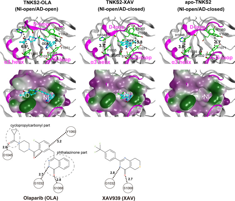
Figure 1 X-ray crystallographic structures of the pocket conformation of tankyrase2-olaparib (TNKS2–OLA) complex, tankyrase2-XAV939 (TNKS2–XAV) complex, and unbound-tankyrase2 (apo-TNKS2). The X-ray crystallographic structures of pocket conformations of the TNKS2–OLA complex, the TNKS2–XAV complex, and apo-TNKS2 are shown in left, center, and right panels, respectively. Top figures show the conformations of the ligand binding pockets. Several key residues (Gly1032, Phe1035, His1048, Tyr1050, Tyr1060, Ser1068, and Tyr1071) are shown using a green stick model. The α3 helix, D-loop, and G-loop regions are shown in magenta. The bound ligands are shown using a ball-and-stick model in cyan. The black dotted lines indicate the distance between the geometric center of the Tyr1050 phenyl ring and that of the Tyr1070 (the ring distance of Tyr1050–Tyr1071) (Å) and the minimum distances between Phe1035 and His1048 (the minimum distance of Phe1035–His1048) (Å). The middle figures show the ligand binding pockets depicted using a molecular surface representation. The hydrophilic and lipophilic regions are drawn in purple and green, respectively. The bottom figures illustrate the structural formula of each ligand. The black dotted lines with numerals represent the distances of hydrogen bonds between the ligand and the amino acids in the binding pocket. AD, adenosine subsite; NI, nicotinamide subsite.
Figure 1 X-ray crystallographic structures of the pocket conformation of tankyrase2-olaparib (TNKS2–OLA) complex, tankyrase2-XAV939 (TNKS2–XAV) complex, and unbound-tankyrase2 (apo-TNKS2). The X-ray crystallographic structures of pocket conformations of the TNKS2–OLA complex, the TNKS2–XAV complex, and apo-TNKS2 are shown in left, center, and right panels, respectively. Top figures show the conformations of the ligand binding pockets. Several key residues (Gly1032, Phe1035, His1048, Tyr1050, Tyr1060, Ser1068, and Tyr1071) are shown using a green stick model. The α3 helix, D-loop, and G-loop regions are shown in magenta. The bound ligands are shown using a ball-and-stick model in cyan. The black dotted lines indicate the distance between the geometric center of the Tyr1050 phenyl ring and that of the Tyr1070 (the ring distance of Tyr1050–Tyr1071) (Å) and the minimum distances between Phe1035 and His1048 (the minimum distance of Phe1035–His1048) (Å). The middle figures show the ligand binding pockets depicted using a molecular surface representation. The hydrophilic and lipophilic regions are drawn in purple and green, respectively. The bottom figures illustrate the structural formula of each ligand. The black dotted lines with numerals represent the distances of hydrogen bonds between the ligand and the amino acids in the binding pocket. AD, adenosine subsite; NI, nicotinamide subsite.CC BY-NC-ND · PubMed Central
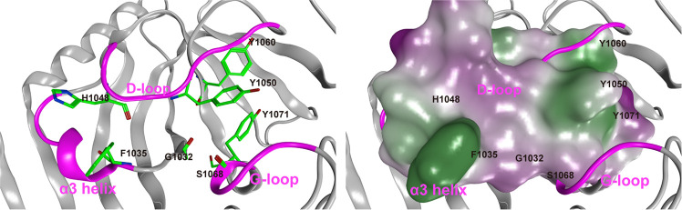
Figure 2 Representative conformation of apo-TNKS2 during the last 550 ns (250–800 ns) of MD trajectory. (Left) The ligand binding pocket is depicted using a ribbon model. Several key residues (Gly1032, Phe1035, His1048, Tyr1050, Tyr1060, Ser1068, and Tyr1071) are shown using a green stick model. The α3 helix, D-loop, and G-loop regions are shown in magenta. The cyan dotted lines indicate the distance between the geometric center of the Tyr1050 phenyl ring and that of the Tyr1070 (the ring distance of Tyr1050–Tyr1071) (Å) and the minimum distance between the Phe1035 and His1048 side chains (heavy atoms; the minimum distance of Phe1035–His1048) (Å). This conformation shows that the NI-closed/AD-closed formed because the AD subsite remained in the closed conformation and the NI subsites became narrow compared to those observed in the experimental structure of apo-TNKS2 (Figure 1 and Table S1). (Right) The ligand binding pocket is depicted using a molecular surface representation. The hydrophilic and lipophilic regions are drawn in purple and green, respectively. These figures are the same view of the structures depicted in Figure 1.
Figure 2 Representative conformation of apo-TNKS2 during the last 550 ns (250–800 ns) of MD trajectory. (Left) The ligand binding pocket is depicted using a ribbon model. Several key residues (Gly1032, Phe1035, His1048, Tyr1050, Tyr1060, Ser1068, and Tyr1071) are shown using a green stick model. The α3 helix, D-loop, and G-loop regions are shown in magenta. The cyan dotted lines indicate the distance between the geometric center of the Tyr1050 phenyl ring and that of the Tyr1070 (the ring distance of Tyr1050–Tyr1071) (Å) and the minimum distance between the Phe1035 and His1048 side chains (heavy atoms; the minimum distance of Phe1035–His1048) (Å). This conformation shows that the NI-closed/AD-closed formed because the AD subsite remained in the closed conformation and the NI subsites became narrow compared to those observed in the experimental structure of apo-TNKS2 (Figure 1 and Table S1). (Right) The ligand binding pocket is depicted using a molecular surface representation. The hydrophilic and lipophilic regions are drawn in purple and green, respectively. These figures are the same view of the structures depicted in Figure 1.CC BY-NC-ND · PubMed Central
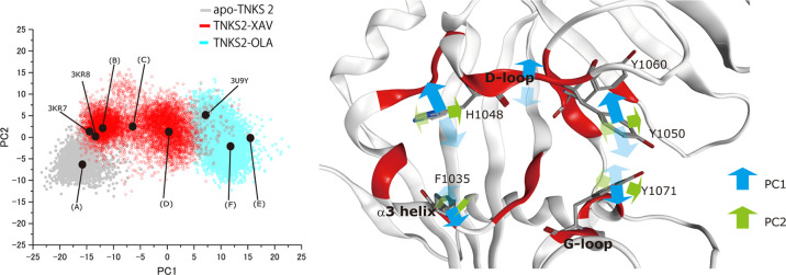
Figure 3 PCA of pocket conformation using MD trajectories of apo-TNKS2, TNKS2–XAV complex, and TNKS2–OLA complex. For the PCA, the first 250 ns of the MD trajectory of apo-TNKS2 and 800 ns trajectories of the TNKS2–XAV complex and the TNKS2–OLA complex were used. The left panel shows the MD trajectories projected onto the plane of the first two components (PC1 and PC2). The contribution ratios of PC1 and PC2 were 44 and 7%, respectively. The black circles represent the projections of the representative conformations of the ligand binding pocket. (A–F) were determined based on the PC1 value histogram shown in Figure 5, and these correspond to conformations of (A–F) of Figure 6. The black circles of 3KR7, 3KR8, and 3U9Y correspond to the ligand-binding pockets of X-ray crystallographic structures of apo-TNKS2, the TNKS2–XAV complex, and the TNKS2–OLA complex. The right panel shows the motions corresponding to the two eigenvectors, respectively. The red regions indicate the position of the 21 amino acid residues used for PCA (see the Methods section). The blue and green arrows represent the motions of PC1 and PC2, respectively.
Figure 3 PCA of pocket conformation using MD trajectories of apo-TNKS2, TNKS2–XAV complex, and TNKS2–OLA complex. For the PCA, the first 250 ns of the MD trajectory of apo-TNKS2 and 800 ns trajectories of the TNKS2–XAV complex and the TNKS2–OLA complex were used. The left panel shows the MD trajectories projected onto the plane of the first two components (PC1 and PC2). The contribution ratios of PC1 and PC2 were 44 and 7%, respectively. The black circles represent the projections of the representative conformations of the ligand binding pocket. (A–F) were determined based on the PC1 value histogram shown in Figure 5, and these correspond to conformations of (A–F) of Figure 6. The black circles of 3KR7, 3KR8, and 3U9Y correspond to the ligand-binding pockets of X-ray crystallographic structures of apo-TNKS2, the TNKS2–XAV complex, and the TNKS2–OLA complex. The right panel shows the motions corresponding to the two eigenvectors, respectively. The red regions indicate the position of the 21 amino acid residues used for PCA (see the Methods section). The blue and green arrows represent the motions of PC1 and PC2, respectively.CC BY-NC-ND · PubMed Central
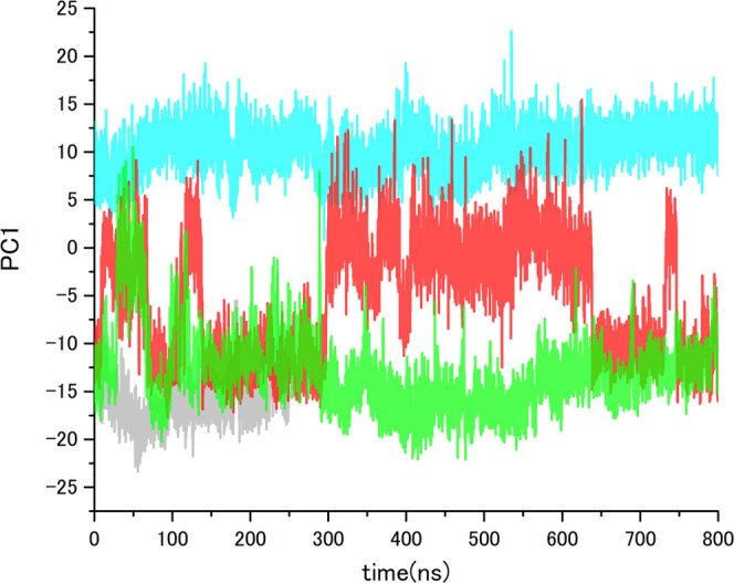
Figure 4 PC1 value time courses of MD trajectories of apo-TNKS2, TNKS2–XAV complex, TNKS2–OLA complex, and apo-TNKS2-CSol. Gray, red, cyan, and green lines indicate the PC1 values of apo-TNKS2, TNKS2–XAV complex, TNKS2–OLA complex, and apo-TNKS2-CSol, respectively. The abscissa is the simulation time (ns), and the ordinate is PC1 value.
Figure 4 PC1 value time courses of MD trajectories of apo-TNKS2, TNKS2–XAV complex, TNKS2–OLA complex, and apo-TNKS2-CSol. Gray, red, cyan, and green lines indicate the PC1 values of apo-TNKS2, TNKS2–XAV complex, TNKS2–OLA complex, and apo-TNKS2-CSol, respectively. The abscissa is the simulation time (ns), and the ordinate is PC1 value.CC BY-NC-ND · PubMed Central
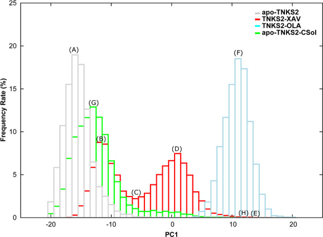
Figure 5 PC1 value histograms of MD simulations of apo-TNKS2, TNKS2–XAV complex, TNKS2–OLA complex, and apo-TNKS2-CSol. Gray, red, cyan, and green boxes indicate the occurrence frequency rate of apo-TNKS2, TNKS2–XAV complex, TNKS2–OLA complex, and apo-TNKS2-CSol, respectively. The abscissa represents the PC1 value, and the ordinate represents the appearance frequency rate (%) of conformations (A–H), thus indicating the representative positions of the respective histograms. (A) The PC1 value peak for apo-TNKS2. (B, D) Two different PC1 value peaks for the TNKS2–XAV complex. (C) The valley between two different PC1 value peaks of the TNKS2–XAV complex. (E) The maximum PC1 value for the TNKS2–XAV complex. (F) The PC1 value peak of the TNKS2–OLA complex. (G, H) The peak and maximum PC1 value of apo-TNKS2-CSol.
Figure 5 PC1 value histograms of MD simulations of apo-TNKS2, TNKS2–XAV complex, TNKS2–OLA complex, and apo-TNKS2-CSol. Gray, red, cyan, and green boxes indicate the occurrence frequency rate of apo-TNKS2, TNKS2–XAV complex, TNKS2–OLA complex, and apo-TNKS2-CSol, respectively. The abscissa represents the PC1 value, and the ordinate represents the appearance frequency rate (%) of conformations (A–H), thus indicating the representative positions of the respective histograms. (A) The PC1 value peak for apo-TNKS2. (B, D) Two different PC1 value peaks for the TNKS2–XAV complex. (C) The valley between two different PC1 value peaks of the TNKS2–XAV complex. (E) The maximum PC1 value for the TNKS2–XAV complex. (F) The PC1 value peak of the TNKS2–OLA complex. (G, H) The peak and maximum PC1 value of apo-TNKS2-CSol.CC BY-NC-ND · PubMed Central
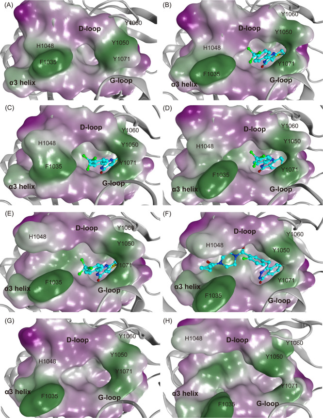
Figure 6 Representative conformations of the ligand binding pocket of MD simulations of apo-TNKS2, TNKS2–XAV complex, TNKS2–OLA complex, and apo-TNKS2-CSol. The conformations (A–H) are labeled with (A–H). The conformations (A–H) in this figure correspond to the positions of (A–H) in Figures 3, 5, and S6. The ligand binding pocket is depicted using molecular surface representations. The hydrophilic and lipophilic regions are drawn in purple and green, respectively. The bound ligands (XAV and OLA) are shown using ball-and-stick models. (A) An apo-TNKS2 conformation (23.3 ns). (B–E) Representative conformations (700.6, 414.5, 580.0, and 549.2 ns, respectively) of the TNKS2–XAV complex. (F) A TNKS2–OLA complex conformation (60.4 ns). Conformations (A–D) exhibit the NI-open/AD-closed form. Conformations (E) and (F) exhibit the NI-open/AD-open form. Conformations (G) and (H) are representative conformations of apo-TNKS2-CSol (616.3 and 49.6 ns), which exhibit the NI-open/AD-closed and NI-open/AD-open forms, respectively.
Figure 6 Representative conformations of the ligand binding pocket of MD simulations of apo-TNKS2, TNKS2–XAV complex, TNKS2–OLA complex, and apo-TNKS2-CSol. The conformations (A–H) are labeled with (A–H). The conformations (A–H) in this figure correspond to the positions of (A–H) in Figures 3, 5, and S6. The ligand binding pocket is depicted using molecular surface representations. The hydrophilic and lipophilic regions are drawn in purple and green, respectively. The bound ligands (XAV and OLA) are shown using ball-and-stick models. (A) An apo-TNKS2 conformation (23.3 ns). (B–E) Representative conformations (700.6, 414.5, 580.0, and 549.2 ns, respectively) of the TNKS2–XAV complex. (F) A TNKS2–OLA complex conformation (60.4 ns). Conformations (A–D) exhibit the NI-open/AD-closed form. Conformations (E) and (F) exhibit the NI-open/AD-open form. Conformations (G) and (H) are representative conformations of apo-TNKS2-CSol (616.3 and 49.6 ns), which exhibit the NI-open/AD-closed and NI-open/AD-open forms, respectively.CC BY-NC-ND · PubMed Central
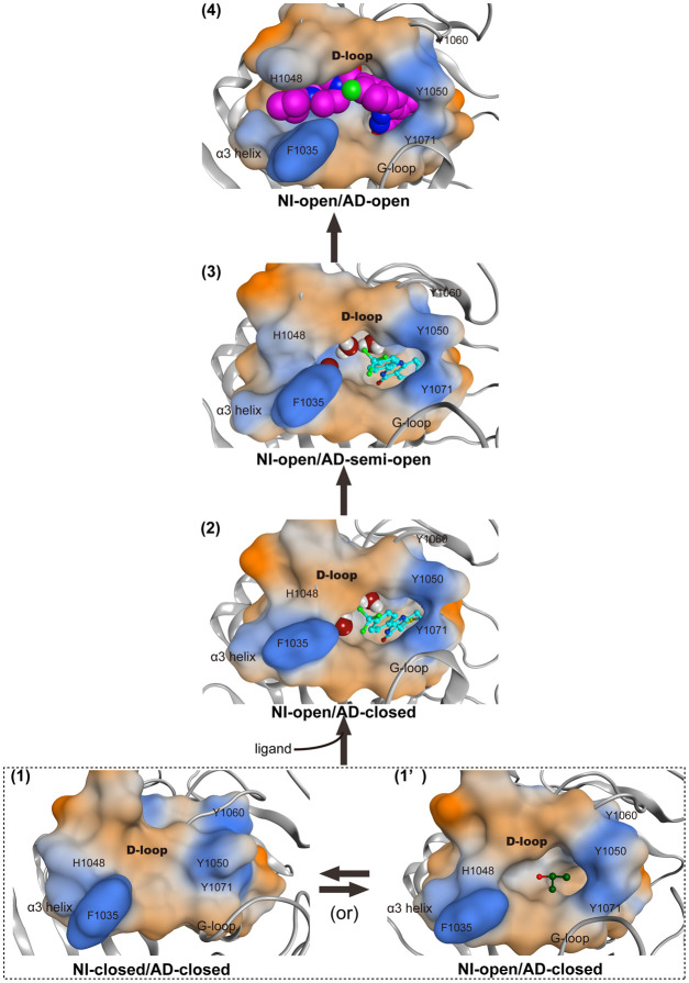
Figure 7 Proposed mechanism of conformational changes of ligand-binding pocket on OLA binding. Four conformations (NI-closed/AD-closed (1), NI-open/AD-closed (1′ and 2), NI-open/AD-semi-open (3), and NI-open/AD-open (4) forms) of the ligand binding pocket of TNKS2 are shown. The dotted box indicates the conformational change between the NI-closed/AD-closed (1) and NI-open/AD-closed (1′) forms of apo-TNKS2. The black arrows indicate the main conformational change pathway of TNKS2 upon OLA binding. The ligand binding pocket is depicted using molecular surface representations. IPA molecule shown in the ball-and-stick model is in the NI-open/AD-closed (1′) form. XAV and water molecules shown in ball-and-stick and space-filling models are in the NI-open/AD-closed (2) and NI-open/AD-semi-open (3) forms, respectively. The OLA molecule shown in space-filling model is in the NI-open/AD-open (4) form. The hydrophilic and lipophilic regions are drawn in orange and blue, respectively.
Figure 7 Proposed mechanism of conformational changes of ligand-binding pocket on OLA binding. Four conformations (NI-closed/AD-closed (1), NI-open/AD-closed (1′ and 2), NI-open/AD-semi-open (3), and NI-open/AD-open (4) forms) of the ligand binding pocket of TNKS2 are shown. The dotted box indicates the conformational change between the NI-closed/AD-closed (1) and NI-open/AD-closed (1′) forms of apo-TNKS2. The black arrows indicate the main conformational change pathway of TNKS2 upon OLA binding. The ligand binding pocket is depicted using molecular surface representations. IPA molecule shown in the ball-and-stick model is in the NI-open/AD-closed (1′) form. XAV and water molecules shown in ball-and-stick and space-filling models are in the NI-open/AD-closed (2) and NI-open/AD-semi-open (3) forms, respectively. The OLA molecule shown in space-filling model is in the NI-open/AD-open (4) form. The hydrophilic and lipophilic regions are drawn in orange and blue, respectively.CC BY-NC-ND · PubMed Central

Verification

Claims the paper makes

The claims and statistics of this paper haven’t been checked yet.

Run the check — free, no account needed. It reads the open-access text and checks the sources it cites.

A few free checks a day · papers already verified open instantly · results are public

Claims other papers make about this one

Each is checked against this paper’s own text: does it say what the citing paper says it does?

Self-check

Percentages, sums and reported differences re-computed from the paper’s own numbers.

The self-check needs the paper’s full text.

Citations

Cites

No references could be resolved yet.

Research works printed but not linked: 43

  1. Hsiao, 2008, Tankyrase function at telomeres, spindle poles, and beyond, Biochimie, 90, 83, 10.1016/j.biochi.2007.07.012 · DOI
  2. Narwal, 2013, Screening and structural analysis of flavones inhibiting tankyrases, J. Med. Chem., 56, 3507, 10.1021/jm3018783 · DOI
  3. Huang, 2009, Tankyrase inhibition stabilizes axin and antagonizes Wnt signalling, Nature, 461, 614, 10.1038/nature08356 · DOI
  4. Narwal, 2012, Structural basis of selective inhibition of human tankyrases, J. Med. Chem., 55, 1360, 10.1021/jm201510p · DOI
  5. Narwal, 2013, Discovery of tankyrase inhibiting flavones with increased potency and isoenzyme selectivity, J. Med. Chem., 56, 7880, 10.1021/jm401463y · DOI
  6. Voronkov, 2013, Structural basis and SAR for G007-LK, a lead stage 1,2,4-triazole based specific tankyrase 1/2 inhibitor, J. Med. Chem., 56, 3012, 10.1021/jm4000566 · DOI
  7. Huang, 2013, Structure-based design of 2-aminopyridine oxazolidinones as potent and selective tankyrase inhibitors, ACS Med. Chem. Lett., 4, 1218, 10.1021/ml4003315 · DOI
  8. Bregman, 2013, Discovery of novel, induced-pocket binding oxazolidinones as potent, selective, and orally bioavailable tankyrase inhibitors, J. Med. Chem., 56, 4320, 10.1021/jm4000038 · DOI
  9. Hua, 2013, Development of novel dual binders as potent, selective, and orally bioavailable tankyrase inhibitors, J. Med. Chem., 56, 10003, 10.1021/jm401317z · DOI
  10. Anumala, 2017, Discovery of a Novel Series of Tankyrase Inhibitors by a Hybridization Approach, J. Med. Chem., 60, 10013, 10.1021/acs.jmedchem.7b00883 · DOI
  11. Schacke, 2019, PARP-1/2 Inhibitor Olaparib Prevents or Partially Reverts EMT Induced by TGF-beta in NMuMG Cells, Int. J. Mol. Sci., 20, 10.3390/ijms20030518 · DOI
  12. Chen, 2009, Small molecule-mediated disruption of Wnt-dependent signaling in tissue regeneration and cancer, Nat. Chem. Biol., 5, 100, 10.1038/nchembio.137 · DOI
  13. Karlberg, 2010, Structural basis for the interaction between tankyrase-2 and a potent Wnt-signaling inhibitor, J. Med. Chem., 53, 5352, 10.1021/jm100249w · DOI
  14. Ruf, 1998, Inhibitor and NAD+ binding to poly­(ADP-ribose) polymerase as derived from crystal structures and homology modeling, Biochemistry, 37, 3893, 10.1021/bi972383s · DOI
  15. Langelier, 2018, NAD­(+) analog reveals PARP-1 substrate-blocking mechanism and allosteric communication from catalytic center to DNA-binding domains, Nat. Commun., 9, 10.1038/s41467-018-03234-8 · DOI
  16. Lehtiö, 2013, Tankyrases as drug targets, FEBS J., 280, 3576, 10.1111/febs.12320 · DOI
  17. Haikarainen, 2014, Tankyrases: structure, function and therapeutic implications in cancer, Curr. Pharm. Des., 20, 6472, 10.2174/1381612820666140630101525 · DOI
  18. Ferri, 2017, Targeting Wnt-driven cancers: Discovery of novel tankyrase inhibitors, Eur. J. Med. Chem., 142, 506, 10.1016/j.ejmech.2017.09.030 · DOI
  19. Gao, 2017, Are induced fit protein conformational changes caused by ligand-binding predictable? A molecular dynamics investigation, J. Comput. Chem., 38, 1229, 10.1002/jcc.24714 · DOI
  20. Berman, 2000, The Protein Data Bank and the challenge of structural genomics, Nat. Struct. Biol., 7, 957, 10.1038/80734 · DOI
  21. Jorgensen, 1983, Morphology of a very extensible insect muscle, Tissue Cell, 15, 639, 10.1016/0040-8166(83)90013-7 · DOI
  22. Kimura, 2017, Deciphering Cryptic Binding Sites on Proteins by Mixed-Solvent Molecular Dynamics, J. Chem. Inf. Model., 57, 1388, 10.1021/acs.jcim.6b00623 · DOI
  23. Beglov, 2018, Exploring the structural origins of cryptic sites on proteins, Proc. Natl. Acad. Sci. U.S.A., 115, E3416, 10.1073/pnas.1711490115 · DOI
  24. An, 2019, Are the Apo Proteins Suitable for the Rational Discovery of Allosteric Drugs?, J. Chem. Inf. Model., 59, 597, 10.1021/acs.jcim.8b00735 · DOI
  25. Berendsen, 1995, Gromacs - a Message-Passing Parallel Molecular-Dynamics Implementation, Comput. Phys. Commun., 91, 43, 10.1016/0010-4655(95)00042-E · DOI
  26. Lindahl, 2001, GROMACS 3.0: a package for molecular simulation and trajectory analysis, J. Mol. Model., 7, 306, 10.1007/s008940100045 · DOI
  27. Van der Spoel, 2005, GROMACS: Fast, flexible, and free, J. Comput. Chem., 26, 1701, 10.1002/jcc.20291 · DOI
  28. Hess, 2008, GROMACS 4: Algorithms for highly efficient, load-balanced, and scalable molecular simulation, J. Chem. Theory Comput., 4, 435, 10.1021/ct700301q · DOI
  29. Pronk, 2013, GROMACS 4.5: a high-throughput and highly parallel open source molecular simulation toolkit, Bioinformatics, 29, 845, 10.1093/bioinformatics/btt055 · DOI
  30. Lindorff-Larsen, 2010, Improved side-chain torsion potentials for the Amber ff99SB protein force field, Proteins, 78, 1950, 10.1002/prot.22711 · DOI
  31. Wang, 2004, Development and testing of a general amber force field, J. Comput. Chem., 25, 1157, 10.1002/jcc.20035 · DOI
  32. Nosé, 1984, A Molecular-Dynamics Method for Simulations in the Canonical Ensemble, Mol. Phys., 52, 255, 10.1080/00268978400101201 · DOI
  33. Parrinello, 1981, Polymorphic Transitions in Single-Crystals - a New Molecular-Dynamics Method, J. Appl. Phys., 52, 7182, 10.1063/1.328693 · DOI
  34. Hess, 1997, LINCS: A linear constraint solver for molecular simulations, J. Comput. Chem., 18, 1463, 10.1002/(SICI)1096-987X(199709)18:12<1463::AID-JCC4>3.0.CO;2-H · DOI
  35. Essmann, 1995, A Smooth Particle Mesh Ewald Method, J. Chem. Phys., 103, 8577, 10.1063/1.470117 · DOI
  36. Jones, 1997, Development and validation of a genetic algorithm for flexible docking, J. Mol. Biol., 267, 727, 10.1006/jmbi.1996.0897 · DOI · Paper page
  37. Verdonk, 2003, Improved protein-ligand docking using GOLD, Proteins, 52, 609, 10.1002/prot.10465 · DOI
  38. Srinivasan, 1998, Continuum Solvent Studies of the Stability of DNA, RNA, and Phosphoramidate–DNA Helices, J. Am. Chem. Soc., 120, 9401, 10.1021/ja981844+ · DOI
  39. Kollman, 2000, Calculating structures and free energies of complex molecules: combining molecular mechanics and continuum models, Acc. Chem. Res., 33, 889, 10.1021/ar000033j · DOI · Paper page
  40. Kuhn, 2005, Validation and use of the MM-PBSA approach for drug discovery, J. Med. Chem., 48, 4040, 10.1021/jm049081q · DOI
  41. Okimoto, 2009, High-performance drug discovery: computational screening by combining docking and molecular dynamics simulations, PLoS Comput. Biol., 5, 10.1371/journal.pcbi.1000528 · DOI
  42. Okimoto, 2018, Use of the Multilayer Fragment Molecular Orbital Method to Predict the Rank Order of Protein-Ligand Binding Affinities: A Case Study Using Tankyrase 2 Inhibitors, ACS Omega, 3, 4475, 10.1021/acsomega.8b00175 · DOI
  43. Connolly, 1983, Analytical molecular surface calculation, J. Appl. Crystallogr., 16, 548, 10.1107/S0021889883010985 · DOI

Cited by

Metadata

Authors
Hirano, Y., Okimoto, N., Fujita, S., & Taiji, M.
Affiliations
RIKEN Center for Biosystems Dynamics Research (BDR) , , 6-2-4 Furuedai , , ,
Venue
ACS Omega
Published
2021-06-29
Volume
6
Issue
27
Pages
17609-17620
ISSN
2470-1343
Cited by
31
References
0
Language
en

About these checks

Registry, retraction, Cites and statistics results are computed, not judged, with one exception: a printed reference that no index lists is read once by a model before it counts as a citation error. Claims are extracted by a model and kept only when their quote appears verbatim in the text; each cited source is then checked, with a model’s help, for whether it says what the claim relies on. Those verdicts can be wrong — read the claim’s quote and the cited source before relying on one.

Statistics and arithmetic are recomputed, not judged.

Confidence bands are shown only for fields calibrated on our annotated test set. None is calibrated yet, so no band is shown.

What counts as a claim ›How we measure confidence ›How we check this ›

Are you an author, or do you see a problem with this page? Request a review

Data sources

Bibliographic data: Semantic Scholar, OpenAlex, Crossref.

Contains information from the Semantic Scholar Academic Graph Datasets, made available under the ODC Attribution License (ODC-BY 1.0).

Semantic Scholar’s data is described in: Kinney, R., et al. (2023). The Semantic Scholar Open Data Platform. arXiv:2301.10140.