Cited by 2

The DOI matches its Crossref record.

Influence of Hydraulic Conductivity Conceptualization and Unsaturated Flow Parameters for an Integrated Hydrological Model

Muñoz‐Vega, Edinsson, Bogena, Heye Reemt, Richard‐Cerda, Juan Carlos, Maxwell, Reed M., Schulz, Stephan·2025·Water Resources Research

Abstract

In recent decades, integrated hydrologic models (IHMs) have advanced our understanding of hydrologic processes across catchment to continental scales. These models couple surface and variably saturated subsurface flow, incorporating land surface models to represent interactions within the critical zone. However, high computational costs hinder calibration and sensitivity analysis. Prior studies show that outputs such as runoff, soil moisture, and energy fluxes are highly sensitive to subsurface parametrization, particularly to the hydraulic conductivity in both saturated and unsaturated zones. Despite its relevance in soil‐vegetation interactions, sensitivity to unsaturated parameters has been less explored, often limited to synthetic domains. To address this, we designed a deterministic approach consisting of 55 simulations, to explore and other parameters sensitivities. We employed the parallel, fully integrated model Parflow‐CLM to simulate water and energy fluxes in a headwater catchment in the Odenwald, Germany. Simulations were evaluated against streamflow and soil moisture observations to ensure realistic results. Multiple combinations of ‐values, anisotropies, and van Genuchten parameters were tested, examining the impact of soil hydraulic properties on plant water uptake. Results show that increasing enhances baseflow and attenuates peak flows, while anisotropy in shallow horizons significantly affects runoff and groundwater dynamics. The shape of the soil water retention curve, represented by the van Genuchten parameters, as well as saturation at field capacity and wilting point, strongly influence simulated soil moisture during dry periods. Overall, our analysis provides insights into subsurface parameter sensitivities to hydrologic responses, supporting the design of calibration schemes for IHM applications.

Overview

The claims and statistics of this paper haven’t been checked yet.

Run the check — free, no account needed. It reads the open-access text and checks the sources it cites.

A few free checks a day · papers already verified open instantly · results are public

Integrity signals

Registry

Crossref · 10.1029/2025wr040785

Cites

Statistics

Figures

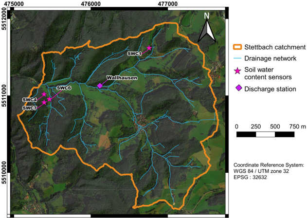
Figure 1 Study area and instrumentation.
Figure 1 Study area and instrumentation.CC-BY · From the PDF
Image 2
CC-BY · From the PDF
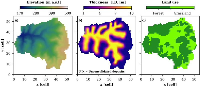
Figure 2 Data used for model geometry (a, b) and land use parameter distribution (c) for the Parflow-CLM models.
Figure 2 Data used for model geometry (a, b) and land use parameter distribution (c) for the Parflow-CLM models.CC-BY · From the PDF
Image 4
CC-BY · From the PDF
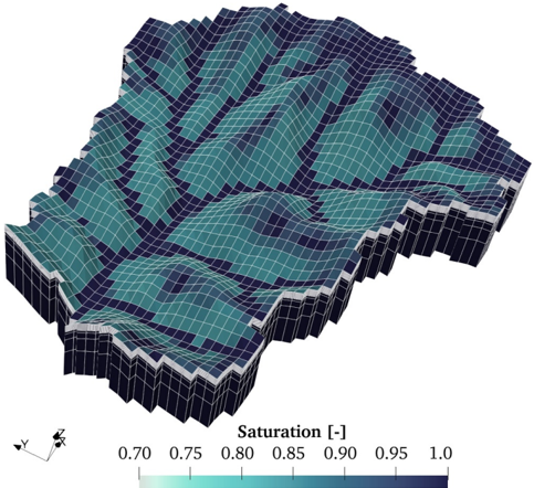
Figure 3 Three-dimensional terrain following grid used for Parflow-CLM models depicting simulated drainage network during a day in winter (7 January 2022). Vertical scale is amplified by a factor of 3 for better visualization.
Figure 3 Three-dimensional terrain following grid used for Parflow-CLM models depicting simulated drainage network during a day in winter (7 January 2022). Vertical scale is amplified by a factor of 3 for better visualization.CC-BY · From the PDF
Image 6
CC-BY · From the PDF
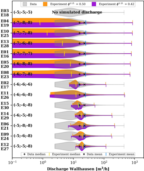
Figure 6 Probability density functions of observed and simulated streamflow distributions at daily resolution for the 15 isotropic conceptual models with both U.D. porosities. Values in parenthesis show the log K [m/s] of the units U.D., weathered rock and Bedrock for each experiment, respectively. Discharges are in logarithmic scale for better visualization of its distribution. For description of the numerical experiments the reader is referred to Table 2.
Figure 6 Probability density functions of observed and simulated streamflow distributions at daily resolution for the 15 isotropic conceptual models with both U.D. porosities. Values in parenthesis show the log K [m/s] of the units U.D., weathered rock and Bedrock for each experiment, respectively. Discharges are in logarithmic scale for better visualization of its distribution. For description of the numerical experiments the reader is referred to Table 2.CC-BY · From the PDF
Image 8
CC-BY · From the PDF
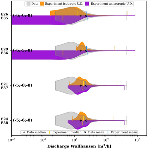
Figure 7 Probability density functions of observed and simulated streamflow distributions at daily resolution for selected isotropic and anisotropic experiments with ϕ U . D . = 0 . 42. Values in parenthesis show the log Kx [m/s] of the units U.D., weathered rock (W.R.) and Bedrock for each case. For anisotropic cases, the units W.R. and Bedrock are isotropic ( Kx = Ky = Kz ) and in U.D. Kx = Ky = 10 Kz . For description of the numerical experiments the reader is referred to Table 2.
Figure 7 Probability density functions of observed and simulated streamflow distributions at daily resolution for selected isotropic and anisotropic experiments with ϕ U . D . = 0 . 42. Values in parenthesis show the log Kx [m/s] of the units U.D., weathered rock (W.R.) and Bedrock for each case. For anisotropic cases, the units W.R. and Bedrock are isotropic ( Kx = Ky = Kz ) and in U.D. Kx = Ky = 10 Kz . For description of the numerical experiments the reader is referred to Table 2.CC-BY · From the PDF
Image 10
CC-BY · From the PDF
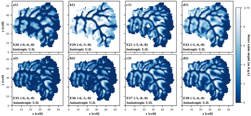
Figure 8 Simulated groundwater table distributions in winter for selected isotropic and anisotropic cases with ϕ U . D . = 0 . 42. Values in parenthesis show the log Kx [m/s] of the units U.D., weathered rock (W.R.) and Bedrock for each case. The units W.R. and Bedrock are isotropic for all models. For anisosotropic simulations, anisotropy is only included in U. D, with Kx = Ky = 10 Kz . For description of the numerical experiments the reader is referred to Table 2.
Figure 8 Simulated groundwater table distributions in winter for selected isotropic and anisotropic cases with ϕ U . D . = 0 . 42. Values in parenthesis show the log Kx [m/s] of the units U.D., weathered rock (W.R.) and Bedrock for each case. The units W.R. and Bedrock are isotropic for all models. For anisosotropic simulations, anisotropy is only included in U. D, with Kx = Ky = 10 Kz . For description of the numerical experiments the reader is referred to Table 2.CC-BY · From the PDF
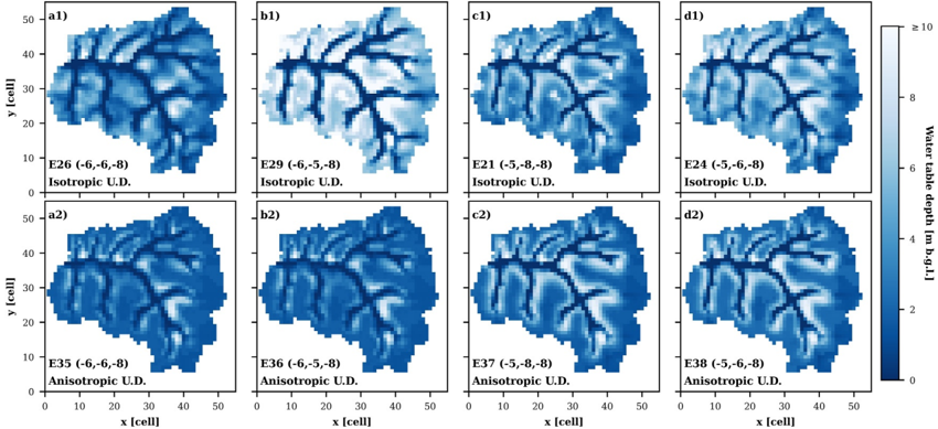
Figure 9 Simulated groundwater table distributions in summer for selected isotropic and anisotropic cases with ϕ U . D . = 0 . 42. Values in parenthesis show the log Kx [m/s] of the units U.D., weathered rock (W.R.) and Bedrock for each case. The units W.R. and Bedrock are isotropic for all models. For anisosotropic simulations, anisotropy is only included in U. D, with Kx = Ky = 10 Kz . For description of the numerical experiments the reader is referred to Table 2.
Figure 9 Simulated groundwater table distributions in summer for selected isotropic and anisotropic cases with ϕ U . D . = 0 . 42. Values in parenthesis show the log Kx [m/s] of the units U.D., weathered rock (W.R.) and Bedrock for each case. The units W.R. and Bedrock are isotropic for all models. For anisosotropic simulations, anisotropy is only included in U. D, with Kx = Ky = 10 Kz . For description of the numerical experiments the reader is referred to Table 2.CC-BY · From the PDF
Image 13
CC-BY · From the PDF
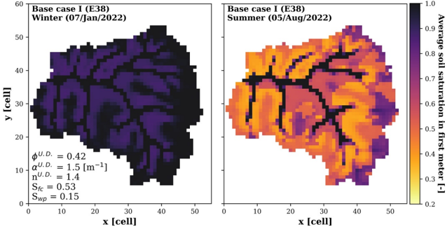
Figure 10 Simulated saturation in the first meter of soil for selected days representing winter and summer conditions for experiment Base case I (E38, Table 2.).
Figure 10 Simulated saturation in the first meter of soil for selected days representing winter and summer conditions for experiment Base case I (E38, Table 2.).CC-BY · From the PDF
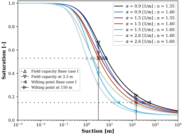
Figure 11 Different cases of van Genuchten parameters, field capacities and wilting points. Note that suction (matric potential) refers to a negative pressure head.
Figure 11 Different cases of van Genuchten parameters, field capacities and wilting points. Note that suction (matric potential) refers to a negative pressure head.CC-BY · From the PDF
Image 16
CC-BY · From the PDF
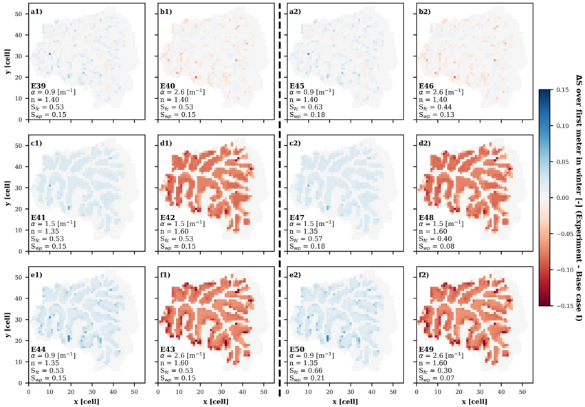
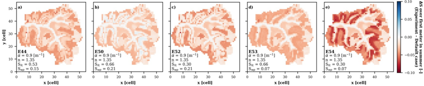
Figure 12 Comparison of average saturations in the first meter of soil in winter. The dashed line divides the cases considering the same S f c and Swp of the Base case I (left) and the ones varying those parameters according to the redefined soil water retention curves (right).
Figure 12 Comparison of average saturations in the first meter of soil in winter. The dashed line divides the cases considering the same S f c and Swp of the Base case I (left) and the ones varying those parameters according to the redefined soil water retention curves (right).CC-BY · From the PDF
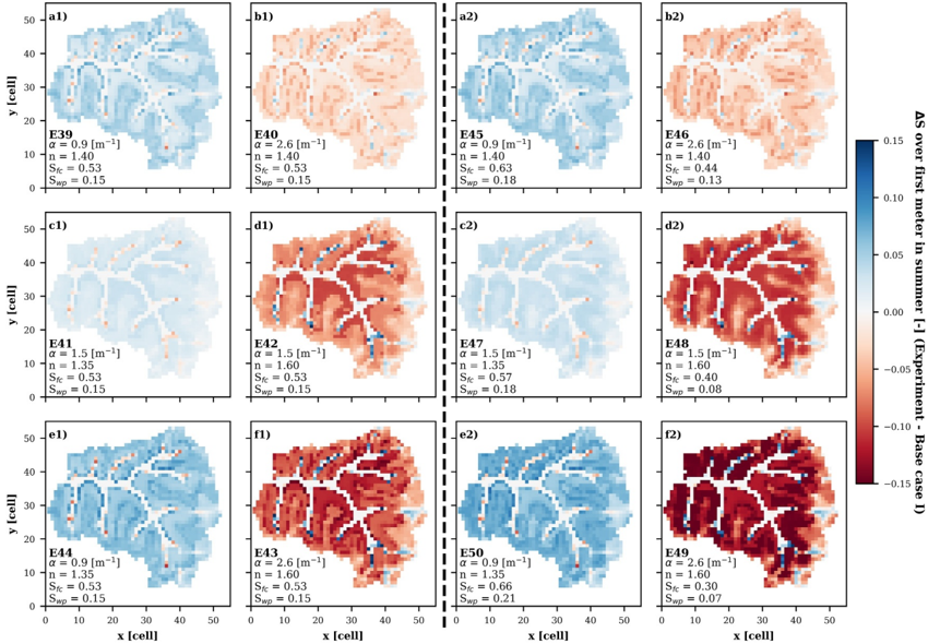
Figure 13 Comparison of average saturation in the first meter of soil in summer. The dashed line divides the cases considering the same S f c and Swp of the Base case I (left) and the ones varying those parameters according to the redefined soil water retention curves (right).
Figure 13 Comparison of average saturation in the first meter of soil in summer. The dashed line divides the cases considering the same S f c and Swp of the Base case I (left) and the ones varying those parameters according to the redefined soil water retention curves (right).CC-BY · From the PDF
Image 19
CC-BY · From the PDF
Image 20
CC-BY · From the PDF
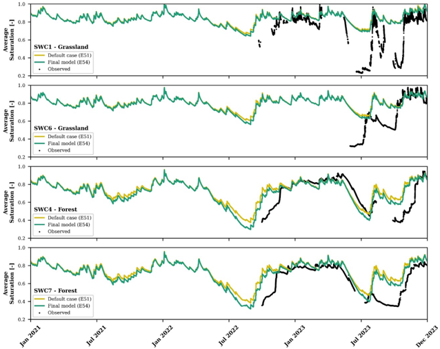
Figure 15 Observed and simulated average soil saturation in first meter for the Default case (E51, S f c = 1 . 0 and Swp = 0 . 1) and for the Final model (E54, S f c = 0 . 30 and Swp = 0 . 07). For description of the numerical experiments the reader is referred to Table 2.
Figure 15 Observed and simulated average soil saturation in first meter for the Default case (E51, S f c = 1 . 0 and Swp = 0 . 1) and for the Final model (E54, S f c = 0 . 30 and Swp = 0 . 07). For description of the numerical experiments the reader is referred to Table 2.CC-BY · From the PDF
Image 22
CC-BY · From the PDF
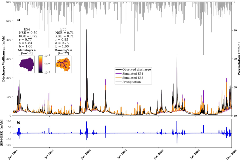
Figure 16 Simulated and observed discharge in Wallhausen at daily resolution for the Final model without and with scaled Manning's coefficients. r, a, and b represent the different components of the Kling-Gupta efficiency.
Figure 16 Simulated and observed discharge in Wallhausen at daily resolution for the Final model without and with scaled Manning's coefficients. r, a, and b represent the different components of the Kling-Gupta efficiency.CC-BY · From the PDF

Verification

Claims the paper makes

The claims and statistics of this paper haven’t been checked yet.

Run the check — free, no account needed. It reads the open-access text and checks the sources it cites.

A few free checks a day · papers already verified open instantly · results are public

Claims other papers make about this one

Each is checked against this paper’s own text: does it say what the citing paper says it does?

Self-check

Percentages, sums and reported differences re-computed from the paper’s own numbers.

The self-check needs the paper’s full text.

Citations

Cites

No references could be resolved yet.

Research works printed but not linked: 54

  1. 10.1007/s00271‐019‐00630‐w · DOI
  2. 10.1007/s10040‐010‐0690‐1 · DOI
  3. 10.1111/gwat.13432 · DOI
  4. 10.2136/vzj2009.0173 · DOI
  5. 10.1002/wrcr.20463 · DOI
  6. 10.3390/s22249792 · DOI
  7. 10.1002/2015wr017039 · DOI
  8. 10.1016/j.envsoft.2023.105824 · DOI
  9. 10.1007/s11242‐015‐0613‐7 · DOI
  10. 10.1029/2019wr026010 · DOI
  11. 10.1007/s00531‐019‐01741‐7 · DOI
  12. 10.1016/j.jhydrol.2018.12.007 · DOI
  13. 10.1029/2023wr035975 · DOI
  14. 10.1016/j.jhydrol.2015.08.011 · DOI
  15. 10.1016/j.jhydrol.2016.03.020 · DOI
  16. 10.1007/s12665‐015‐5041‐z · DOI
  17. 10.1002/hyp.13327 · DOI
  18. 10.1016/j.jhydrol.2009.08.003 · DOI · Paper page
  19. 10.1002/vzj2.20163 · DOI
  20. HVBG, 2024, Digitale topographische karte 1:25 000 (dtk25)
  21. HVBG, 2024, Digitales geländemodell (dgm1)
  22. 10.1016/j.catena.2022.106281 · DOI
  23. 10.1016/j.jhydrol.2019.04.094 · DOI
  24. 10.1016/j.cageo.2015.07.001 · DOI
  25. 10.1016/j.jhydrol.2015.12.002 · DOI
  26. 10.1088/1748‐9326/4/3/035007 · DOI
  27. 10.1016/j.advwatres.2005.08.006 · DOI
  28. 10.1175/jhm‐d‐23‐0140.1 · DOI
  29. 10.5194/gmd‐13‐1373‐2020 · DOI
  30. 10.1007/s10040‐021‐02339‐7 · DOI
  31. 10.1029/2020wr027326 · DOI
  32. 10.1016/j.jhydrol.2024.131542 · DOI
  33. 10.5194/hess‐24‐2437‐2020 · DOI
  34. 10.1016/j.advwatres.2012.10.001 · DOI
  35. 10.1002/2013wr013725 · DOI
  36. 10.1029/2003wr002721 · DOI
  37. 10.5194/hess‐11‐1633‐2007 · DOI
  38. 10.1029/2020wr027714 · DOI
  39. 10.1029/2010wr009111 · DOI
  40. 10.1029/2008wr006908 · DOI
  41. 10.1029/2005rg000169 · DOI
  42. 10.1002/hyp.13448 · DOI
  43. 10.1007/s12665‐013‐2342‐y · DOI
  44. 10.1016/j.advwatres.2017.02.010 · DOI
  45. 10.1002/2014wr016371 · DOI
  46. 10.1029/2011wr011149 · DOI
  47. 10.1007/s10040‐024‐02773‐3 · DOI
  48. 10.1016/j.jhydrol.2022.127991 · DOI
  49. 10.1016/j.jhydrol.2014.10.020 · DOI
  50. 10.1007/s007100170024 · DOI
  51. 10.2136/sssaj1980.03615995004400050002x · DOI · Paper page
  52. 10.1016/j.jhydrol.2013.11.061 · DOI · Paper page
  53. 10.2136/vzj2010.0045 · DOI
  54. 10.1016/j.jhydrol.2017.01.004 · DOI

Metadata

Authors
Muñoz‐Vega, E., Bogena, H. R., Richard‐Cerda, J. C., Maxwell, R. M., & Schulz, S.
Affiliations
  • Technische Universität Darmstadt Institute of Applied Geosciences Darmstadt Germany
  • Forschungszentrum Jülich GmbH Institute of Bio‐ and Geosciences Agrosphere Institute (IBG‐3) Jülich Germany
  • Department of Civil and Environmental Engineering Princeton University Princeton NJ USA
Venue
Water Resources Research
Published
2025-11
Volume
61
Issue
11
ISSN
  • 0043-1397
  • 1944-7973
Cited by
2
References
0
Language
en
Funders
Deutsche Forschungsgemeinschaft (459684982)

About these checks

Registry, retraction, Cites and statistics results are computed, not judged, with one exception: a printed reference that no index lists is read once by a model before it counts as a citation error. Claims are extracted by a model and kept only when their quote appears verbatim in the text; each cited source is then checked, with a model’s help, for whether it says what the claim relies on. Those verdicts can be wrong — read the claim’s quote and the cited source before relying on one.

Statistics and arithmetic are recomputed, not judged.

Confidence bands are shown only for fields calibrated on our annotated test set. None is calibrated yet, so no band is shown.

What counts as a claim ›How we measure confidence ›How we check this ›

Are you an author, or do you see a problem with this page? Request a review