Cited by 12Advanced Electron Microscopy Techniques and ApplicationsEnzyme Structure and FunctionProtein Structure and Dynamics

The DOI matches its Crossref record; 3 of the 3 references it cites were found in a registry or an index.

CryoPROS: Correcting misalignment caused by preferred orientation using AI-generated auxiliary particles

Open access

Published version of a preprint

Abstract

Abstract The preferred orientation phenomenon is a common issue in cryo-EM, posing a persistent challenge to conventional reconstruction methods. In this study, we introduce CryoPROS, a computational framework designed to correct misalignment caused by preferred orientation through co-refining the raw and auxiliary particles. These auxiliary particles, generated using a self-supervised deep generative model, enhance the alignment accuracy of particles in datasets affected by preferred orientation. CryoPROS achieved near-atomic resolution with the untilted HA-trimer dataset and successfully resolved high-resolution structures from three experimental datasets, including P001-Y, Na\textsubscript{\textsl{X}}, and hormone-sensitive lipase dimer, all affected by preferred orientation issues. Extensive experiments validate the robustness of cryoPROS and its minimal risk of introducing model bias. These findings suggest that in many cases thought to suffer from preferred orientation, addressing misalignment issues can lead to significant improvements in the density map.

Overview

The claims and statistics of this paper haven’t been checked yet.

Run the check — free, no account needed. It reads the open-access text and checks the sources it cites.

A few free checks a day · papers already verified open instantly · results are public

Integrity signals

Registry

Crossref · 10.1038/s41467-025-59797-w

Cites

3 of 3 references verified0 citation errors · 0 not checkable

Statistics

Figures

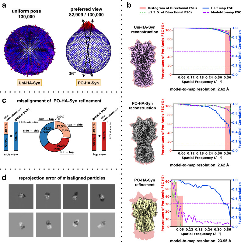
Fig. 1 Misalignment on structural determination in preferential oriented datasets. a Pose distribution of Uni-HA-Syn (left) and PO-HA-Syn (right) datasets. b Comparison of density maps for the Uni-HA-Syn reconstruction (top), PO-HA-Syn reconstruction (middle), and PO-HA-Syn auto refinement (bottom). Density map quality metrics for each density map are shown to the right. The global half-maps FSC is plotted as a solid blue line, and the map-to-model FSC is shown as a dotted purple line. The green shaded area (bounded by dotted green lines) indicates the spread of directional resolution values, defined as the mean ±1 standard deviation (SD). The light coral region represents the histogram of directional FSCs. c Particle misalignments in PO-HA-Syn auto refinement. d Visualization of reprojection error between auto refinement estimates and ground-truth orientations for selected particles.
Fig. 1 Misalignment on structural determination in preferential oriented datasets. a Pose distribution of Uni-HA-Syn (left) and PO-HA-Syn (right) datasets. b Comparison of density maps for the Uni-HA-Syn reconstruction (top), PO-HA-Syn reconstruction (middle), and PO-HA-Syn auto refinement (bottom). Density map quality metrics for each density map are shown to the right. The global half-maps FSC is plotted as a solid blue line, and the map-to-model FSC is shown as a dotted purple line. The green shaded area (bounded by dotted green lines) indicates the spread of directional resolution values, defined as the mean ±1 standard deviation (SD). The light coral region represents the histogram of directional FSCs. c Particle misalignments in PO-HA-Syn auto refinement. d Visualization of reprojection error between auto refinement estimates and ground-truth orientations for selected particles.CC BY-NC-ND · PubMed Central
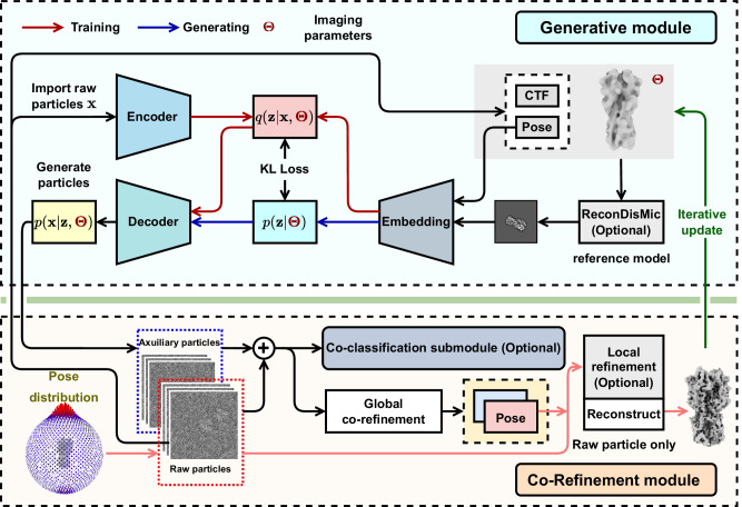
Fig. 2 The workflow of cryoPROS. The cryoPROS protocol includes two components: generative module and co-refinement module. Using imaging parameters Θ, the generative module trains three networks: the encoding network q(z∣Θ,), the prior network p(z∣Θ), and the decoding network p(x∣z,Θ). After training, this module can generate auxiliary particles through p(z∣Θ) and p(x∣z,Θ), indicated by a blue arrow. Additionally, the optional ReconDisMic algorithm can be employed to generate micelles in studies involving membrane proteins. The co-refinement module employs cryo-EM single-particle analysis software for global co-refinement with both raw and auxiliary particles, estimating the pose parameters for the raw particles. Optionally, these pose parameters can be further refined through a local refinement step. Co-classification can also be adopted with existing single-particle analysis software. The refined pose parameters are then utilized to reconstruct a volume for subsequent iterations.
Fig. 2 The workflow of cryoPROS. The cryoPROS protocol includes two components: generative module and co-refinement module. Using imaging parameters Θ, the generative module trains three networks: the encoding network q(z∣Θ,), the prior network p(z∣Θ), and the decoding network p(x∣z,Θ). After training, this module can generate auxiliary particles through p(z∣Θ) and p(x∣z,Θ), indicated by a blue arrow. Additionally, the optional ReconDisMic algorithm can be employed to generate micelles in studies involving membrane proteins. The co-refinement module employs cryo-EM single-particle analysis software for global co-refinement with both raw and auxiliary particles, estimating the pose parameters for the raw particles. Optionally, these pose parameters can be further refined through a local refinement step. Co-classification can also be adopted with existing single-particle analysis software. The refined pose parameters are then utilized to reconstruct a volume for subsequent iterations.CC BY-NC-ND · PubMed Central
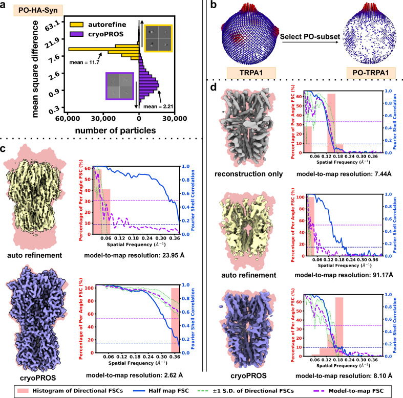
Fig. 3 Correcting misalignment with cryoPROS on PO-HA-Syn and PO-TRPA1 datasets. a Histograms showing the mean square differences between ground truth projections and estimated reprojections from cryoPROS and conventional autorefine for the PO-HA-Syn dataset. b Pose distributions for TRPA1 and PO-TRPA1 datasets. c Comparison of reconstructed density maps and FSCs between conventional autorefine (top) and cryoPROS (bottom) for the PO-HA-Syn dataset. d Comparison of density maps obtained by reconstruction only (top), autorefine (middle), and cryoPROS (bottom) for the PO-TRPA1 dataset. Density maps in panel (c, d) are overlaid on backgrounds derived from their ground truth atomic models (in magenta). Density map quality metrics for each density map are shown to the right. The global half-maps FSC is plotted as a solid blue line, and the map-to-model FSC is shown as a dotted purple line. The green shaded area (bounded by dotted green lines) indicates the spread of directional resolution values, defined as the mean ±1 standard deviation (SD). The light coral region represents the histogram of directional FSCs.
Fig. 3 Correcting misalignment with cryoPROS on PO-HA-Syn and PO-TRPA1 datasets. a Histograms showing the mean square differences between ground truth projections and estimated reprojections from cryoPROS and conventional autorefine for the PO-HA-Syn dataset. b Pose distributions for TRPA1 and PO-TRPA1 datasets. c Comparison of reconstructed density maps and FSCs between conventional autorefine (top) and cryoPROS (bottom) for the PO-HA-Syn dataset. d Comparison of density maps obtained by reconstruction only (top), autorefine (middle), and cryoPROS (bottom) for the PO-TRPA1 dataset. Density maps in panel (c, d) are overlaid on backgrounds derived from their ground truth atomic models (in magenta). Density map quality metrics for each density map are shown to the right. The global half-maps FSC is plotted as a solid blue line, and the map-to-model FSC is shown as a dotted purple line. The green shaded area (bounded by dotted green lines) indicates the spread of directional resolution values, defined as the mean ±1 standard deviation (SD). The light coral region represents the histogram of directional FSCs.CC BY-NC-ND · PubMed Central
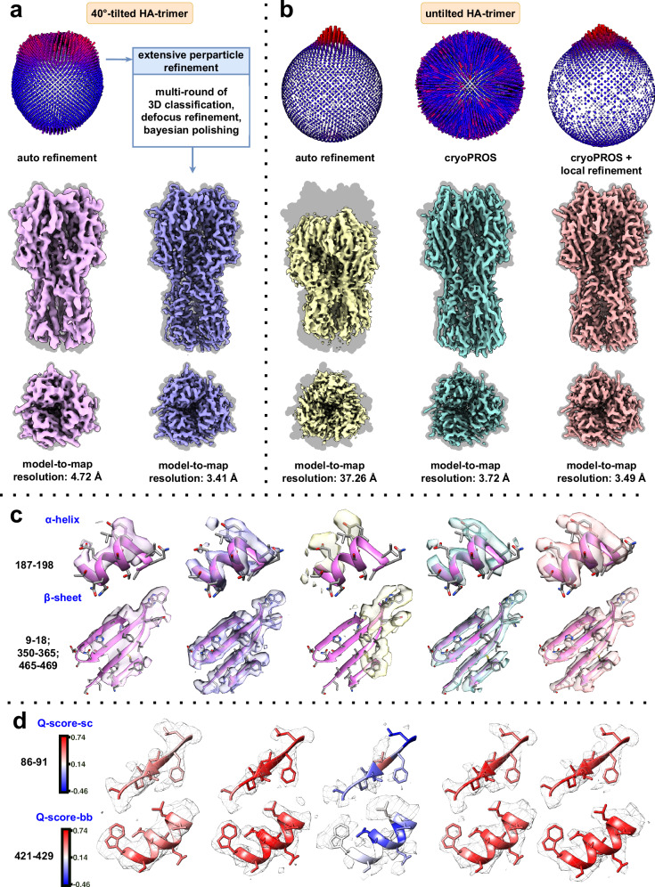
Fig. 4 CryoPROS enables near-atomic resolution recovery from an untilted dataset of highly preferentially oriented HA trimer. a Pose distribution and reconstructed density maps of the tilt-collected dataset, showing autorefinement (left) and state-of-the-art results (right). b Pose distribution and reconstructed density maps of the untilted dataset, comparing autorefinement (left), cryoPROS (middle), and cryoPROS with local refinement (right). Density maps in (a, b) are overlaid on backgrounds derived from their ground truth atomic models (in gray). c Close-up views of selected regions from the density maps, highlighting the α-helix (top) and β-sheet (bottom). d Selected regions in gray mesh style, with the embedded atomic model colored by average Q-score.sc and Q-score.bb values, respectively.
Fig. 4 CryoPROS enables near-atomic resolution recovery from an untilted dataset of highly preferentially oriented HA trimer. a Pose distribution and reconstructed density maps of the tilt-collected dataset, showing autorefinement (left) and state-of-the-art results (right). b Pose distribution and reconstructed density maps of the untilted dataset, comparing autorefinement (left), cryoPROS (middle), and cryoPROS with local refinement (right). Density maps in (a, b) are overlaid on backgrounds derived from their ground truth atomic models (in gray). c Close-up views of selected regions from the density maps, highlighting the α-helix (top) and β-sheet (bottom). d Selected regions in gray mesh style, with the embedded atomic model colored by average Q-score.sc and Q-score.bb values, respectively.CC BY-NC-ND · PubMed Central
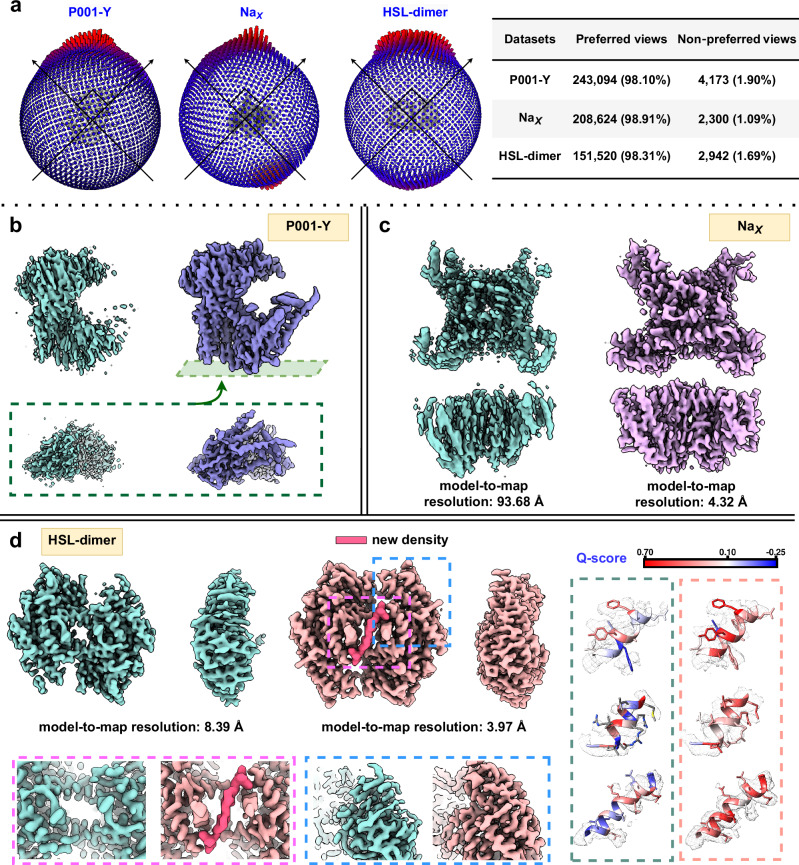
Fig. 5 CryoPROS enables structure determination for three preferentially oriented experimental datasets. a Pose distributions for the three experimental datasets: P001-Y (left), NaX (middle), and HSL-dimer (right), showing the proportion of particles in preferred and non-preferred orientations. b Comparison of density maps from conventional refinement (cyan) and cryoPROS (violet) for the P001-Y dataset. c Comparison of density maps from conventional refinement (cyan) and cryoPROS (pink) for the NaX dataset. d Density maps of HSL-dimer from conventional refinement (cyan) and cryoPROS (magenta), with enlarged views highlighting conformational differences at the central interface (pink box) and prominent α-helix features (blue box). Close-up views of selected regions from HSL-dimer density maps, comparing conventional refinement (left) and cryoPROS (right), are shown with embedded atomic models colored by Q-score.
Fig. 5 CryoPROS enables structure determination for three preferentially oriented experimental datasets. a Pose distributions for the three experimental datasets: P001-Y (left), NaX (middle), and HSL-dimer (right), showing the proportion of particles in preferred and non-preferred orientations. b Comparison of density maps from conventional refinement (cyan) and cryoPROS (violet) for the P001-Y dataset. c Comparison of density maps from conventional refinement (cyan) and cryoPROS (pink) for the NaX dataset. d Density maps of HSL-dimer from conventional refinement (cyan) and cryoPROS (magenta), with enlarged views highlighting conformational differences at the central interface (pink box) and prominent α-helix features (blue box). Close-up views of selected regions from HSL-dimer density maps, comparing conventional refinement (left) and cryoPROS (right), are shown with embedded atomic models colored by Q-score.CC BY-NC-ND · PubMed Central
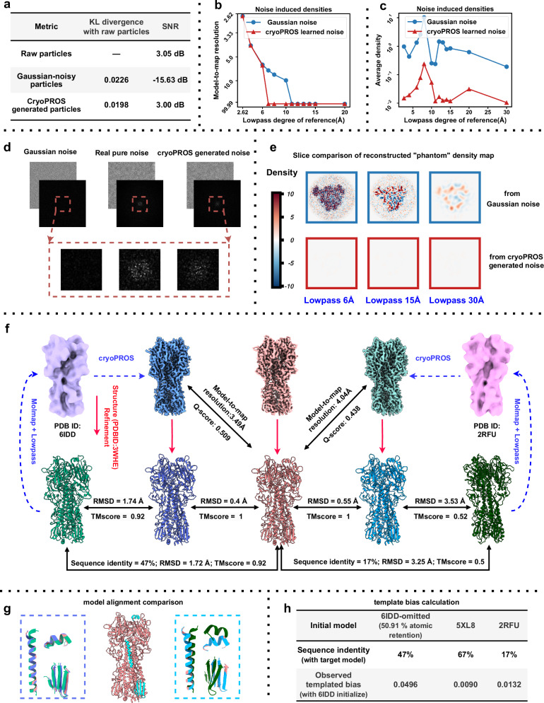
Fig. 6 Model bias risk analysis of cryoPROS. a Evaluation of similarity between raw particles and generated noisy particles (including Gaussian-noisy and cryoPROS-generated noisy particles) using KL divergence and SNR. b Model-to-map resolution of “phantom” density maps from the “Einstein from noise” experiment, with autorefinement performed on Gaussian and cryoPROS noise stacks using varying degrees of lowpass-filtered density maps (ribosome, PDB ID: 6PCQ) as references. c Comparison of average densities from the “Einstein from noise” experiment. d Comparison of Gaussian, real, and cryoPROS-generated noise, with power spectral density plots and an enlarged view of low frequencies (red box). e Slice comparison of “phantom” density maps from the “Einstein from noise” experiment, showing results from Gaussian and cryoPROS-generated noise with different levels of lowpass-filtered homologous proteins. f Structure refinement results using different homologous proteins: cryoPROS-6IDD and cryoPROS-2RFU. 6IDD (light green atomic model, light purple density) and 2RFU (dark green atomic model, pink density) are shown on the left and right, with cryoPROS-6IDD (dark blue), tilt-collected (red), and cryoPROS-2RFU (cyan) densities in the middle. Structure-refined models are below. Similarity was assessed using RMSD and TM-score. g Atomic model alignment for cryoPROS-6IDD and cryoPROS-2RFU, focusing on selected regions, with colors matching panel (f). h Template bias assessment using cisTEM’s measure_template_bias script, with 6IDD as the baseline.
Fig. 6 Model bias risk analysis of cryoPROS. a Evaluation of similarity between raw particles and generated noisy particles (including Gaussian-noisy and cryoPROS-generated noisy particles) using KL divergence and SNR. b Model-to-map resolution of “phantom” density maps from the “Einstein from noise” experiment, with autorefinement performed on Gaussian and cryoPROS noise stacks using varying degrees of lowpass-filtered density maps (ribosome, PDB ID: 6PCQ) as references. c Comparison of average densities from the “Einstein from noise” experiment. d Comparison of Gaussian, real, and cryoPROS-generated noise, with power spectral density plots and an enlarged view of low frequencies (red box). e Slice comparison of “phantom” density maps from the “Einstein from noise” experiment, showing results from Gaussian and cryoPROS-generated noise with different levels of lowpass-filtered homologous proteins. f Structure refinement results using different homologous proteins: cryoPROS-6IDD and cryoPROS-2RFU. 6IDD (light green atomic model, light purple density) and 2RFU (dark green atomic model, pink density) are shown on the left and right, with cryoPROS-6IDD (dark blue), tilt-collected (red), and cryoPROS-2RFU (cyan) densities in the middle. Structure-refined models are below. Similarity was assessed using RMSD and TM-score. g Atomic model alignment for cryoPROS-6IDD and cryoPROS-2RFU, focusing on selected regions, with colors matching panel (f). h Template bias assessment using cisTEM’s measure_template_bias script, with 6IDD as the baseline.CC BY-NC-ND · PubMed Central

Verification

Claims the paper makes

The claims and statistics of this paper haven’t been checked yet.

Run the check — free, no account needed. It reads the open-access text and checks the sources it cites.

A few free checks a day · papers already verified open instantly · results are public

Self-check

Percentages, sums and reported differences re-computed from the paper’s own numbers.

The self-check needs the paper’s full text.

Citations

Cites

Research works printed but not linked: 44

  1. Cheng, Y. Single-particle cryo-EM—How did it get here and where will it go. Science 361, 876–880 (2018). · DOI
  2. Lyumkis, D. Challenges and opportunities in cryo-EM single-particle analysis. J. Biol. Chem. 294, 5181–5197 (2019). · DOI
  3. Glaeser, R. M. & Han, B.-G. Opinion: hazards faced by macromolecules when confined to thin aqueous films. Biophys. Rep. 3, 1–7 (2017). · DOI
  4. Tan, Y. Z. et al. Addressing preferred specimen orientation in single-particle cryo-EM through tilting. Nat. Methods 14, 793–796 (2017). · DOI
  5. Glaeser, R. M. How good can cryo-EM become? Nat. Methods 13, 28–32 (2016). · DOI
  6. Boisset, N. et al. Overabundant single-particle electron microscope views induce a three-dimensional reconstruction artifact. Ultramicroscopy 74, 201–207 (1998). · DOI
  7. Barth, M., Bryan, R. K. & Hegerl, R. Approximation of missing-cone data in 3D electron microscopy. Ultramicroscopy 31, 365–378 (1989). · DOI
  8. Drulyte, I. et al. Approaches to altering particle distributions in cryo-electron microscopy sample preparation. Acta Crystallogr. Sect. D. 74, 560–571 (2018). · DOI
  9. Noble, A. J. et al. Routine single particle CryoEM sample and grid characterization by tomography. eLife 7, e34257 (2018). · DOI
  10. Baldwin, P. R. & Lyumkis, D. Tools for visualizing and analyzing Fourier space sampling in Cryo-EM. Prog. Biophys. Mol. Biol. 160, 53–65 (2021). · DOI
  11. Baldwin, P. & Lyumkis, D. Non-uniformity of projection distributions attenuates resolution in Cryo-EM. Prog. Biophys. Mol. Biol. 150, 160–183 (2020). · DOI
  12. Hauer, F. et al. GraDeR: Membrane Protein Complex Preparation for Single-Particle Cryo-EM. Structure 23, 1769–1775 (2015). · DOI
  13. Chen, J. et al. Eliminating effects of particle adsorption to the air/water interface in single-particle cryo-electron microscopy: Bacterial RNA polymerase and CHAPSO. J. Struct. Biol. X. 1, 100005 (2019).
  14. Li, B. et al. Effect of charge on protein preferred orientation at the air–water interface in cryo-electron microscopy. J. Struct. Biol. 213, 107783 (2021). · DOI
  15. Frotscher, E. et al. A fluorinated detergent for membrane-protein applications. Angew. Chem. 54, 5069–5073 (2015). · DOI
  16. Neselu, K. et al. Measuring the effects of ice thickness on resolution in single particle cryo-EM. J. Struct. Biol. X, 100085 (2023).
  17. Noble, A. J. et al. Reducing effects of particle adsorption to the air–water interface in cryo-EM. Nat. Methods 15, 793–795 (2018). · DOI
  18. Bromberg, R. et al. The His-tag as a decoy modulating preferred orientation in cryoEM. Front. Mol. Biosci.9, 912072 (2022). · DOI
  19. Wu, K. et al. Application of monolayer graphene and its derivative in Cryo-EM sample preparation. Int. J. Mol. Sci. 2021. 22, https://doi.org/10.3390/ijms22168940. · DOI
  20. Xu, J. et al. Structural engineering of graphene for high‐resolution cryo‐electron microscopy. SmartMat 2, 202–212 (2021). · DOI
  21. Zivanov, J. et al. New tools for automated high-resolution cryo-EM structure determination in RELION-3. eLife. 7, e42166 (2018). · DOI
  22. Aiyer, S. et al. Overcoming resolution attenuation during tilted cryo-EM data collection. Nat. Commun. 15, 389 (2024). · DOI
  23. Rosenthal, P. B. & Henderson, R. Optimal determination of particle orientation, absolute hand, and contrast loss in single-particle electron cryomicroscopy. J. Mol. Biol. 333, 721–745 (2003) · DOI · Paper page
  24. Zheng, D. et al. Learn from unpaired data for image restoration: A variational bayes approach. IEEE Trans. Pattern Anal. Mach. Intell. 45, 5889–5903 (2022).
  25. Zheng, D. et al. SeNM-VAE: Semi-supervised noise modeling with hierarchical variational autoencoder. in 2024 IEEE/CVF Conference on Computer Vision and Pattern Recognition (CVPR). 2024. · DOI
  26. Zivanov, J., Nakane, T. & Scheres, S. H. W. A Bayesian approach to beam-induced motion correction in cryo-EM single-particle analysis. IUCrJ 6, 5–17 (2019). · DOI
  27. Hu, M. et al. A particle-filter framework for robust cryo-EM 3D reconstruction. Nat. Methods 15, 1083–1089 (2018). · DOI
  28. Lin, W.-C. et al. Clustering-based undersampling in class-imbalanced data. Inf. Sci. 409-410, 17–26 (2017). · DOI · Paper page
  29. Batista, G. E. A. P. A., Prati, R. C. & Monard, M. C. A study of the behavior of several methods for balancing machine learning training data. SIGKDD Explor. Newsl. 6, 20–29 (2004). · DOI
  30. Sun, Z. et al. A novel ensemble method for classifying imbalanced data. Pattern Recognit. 48, 1623–1637 (2015). · DOI
  31. Sorzano, C. O. S. et al. A clustering approach to multireference alignment of single-particle projections in electron microscopy. J. Struct. Biol. 171, 197–206 (2010). · DOI
  32. Sorzano, C. O. S. et al. Algorithmic robustness to preferred orientations in single particle analysis by CryoEM. J. Struct. Biol. 213, 107695 (2021). · DOI
  33. Sorzano, C. O. S. et al. On bias, variance, overfitting, gold standard and consensus in single-particle analysis by cryo-electron microscopy. Acta Crystallogr. Sect. D. 78, 410–423 (2022). · DOI
  34. Grant, T., Rohou, A. & Grigorieff, N. cisTEM, user-friendly software for single-particle image processing. eLife 7, e35383 (2018). · DOI
  35. He, J., Li, T. & Huang, S.-Y. Improvement of cryo-EM maps by simultaneous local and non-local deep learning. Nat. Commun. 14, 3217 (2023). · DOI
  36. Paulsen, C. E. et al. Structure of the TRPA1 ion channel suggests regulatory mechanisms. Nature 525, 552–552 (2015). · DOI
  37. Bepler, T. et al. Topaz-Denoise: general deep denoising models for cryoEM and cryoET. Nat. Commun. 11, 5208 (2020). · DOI
  38. Henderson, R. Avoiding the pitfalls of single particle cryo-electron microscopy: Einstein from noise. Proc. Natl Acad. Sci. 110, 18037–18041 (2013). · DOI
  39. Punjani, A. & Fleet, D. J. 3DFlex: Determining structure and motion of flexible proteins from cryo-EM. Nat. Methods 20, 860–870 (2023). · DOI
  40. Child, R. Very Deep VAEs Generalize Autoregressive Models and Can Outperform Them on Images. Preprint at https://doi.org/10.48550/arXiv.2011.10650 (2021). · DOI · Paper page
  41. Vahdat, A. & Kautz, J. NVAE: A Deep Hierarchical Variational Autoencoder. Preprint at https://doi.org/10.48550/arXiv.2007.03898 (2021). · DOI
  42. Sønderby, C. K. et al., Ladder variational autoencoders, in Proceedings of the 30th International Conference on Neural Information Processing Systems. 2016, Curran Associates Inc.: Barcelona, Spain. p. 3745–3753.
  43. Zhang, Y. et al. Residual dense network for image super-resolution. In Proceedings of the IEEE Conference on Computer Vision and Pattern Recognition (CVPR), 2472–2481 (2018). · DOI
  44. Kingma, D. P. & Ba, J. Adam: A method for stochastic optimization. Preprint at https://arxiv.org/abs/1412.6980. · arXiv

Metadata

Authors
Zhang, H., Zheng, D., Wu, Q., Yan, N., Peng, H., Hu, Q., Peng, Y., Yan, Z., Shi, Z., Bao, C., & Hu, M.
Affiliations
  • Tsinghua University (CN)
  • University of California, San Francisco (US)
  • Center for Life Sciences (CN)
  • Westlake University (CN)
  • Hunan University (CN)
  • Beijing Institute of Mathematical Sciences and Applications (CN)
  • State Key Laboratory of Membrane Biology (CN)
  • Shenzhen Medical Academy of Research and Translation (CN)
Corresponding author
  • Bao, Chenglong
  • Hu, Mingxu
Venue
Nature Communications
Published
2025-05-16
Volume
16
Issue
1
Pages
4565-4565
ISSN
2041-1723 (ISSN-L)
OpenAlex
W4410438894
Cited by
12
References
3
Citations by year
2026: 7 · 2025: 5
FWCI
4.32
Type
journal article
Language
en
Open access
Locations
  • Nature Communications (publishedVersion, cc-by-nc-nd)
  • Research Square (acceptedVersion, cc-by)
  • PubMed Central (publishedVersion, cc-by-nc-nd)
  • PubMed (publishedVersion)
  • RePEc: Research Papers in Economics (submittedVersion)
  • DOAJ (DOAJ: Directory of Open Access Journals) (submittedVersion, cc-by-sa)
Funders
  • National Natural Science Foundation of China (12271291, 12071244)
  • National Key R&D Program of China
  • Beijing Frontier Research Center for Biological Structure, Shenzhen Medical Academy of Research and Translation
Topics
  • Life Sciences › Biochemistry, Genetics and Molecular Biology › Structural Biology › Advanced Electron Microscopy Techniques and Applications
  • Life Sciences › Biochemistry, Genetics and Molecular Biology › Structural Biology › Enzyme Structure and Function
  • Life Sciences › Biochemistry, Genetics and Molecular Biology › Molecular Biology › Protein Structure and Dynamics
Keywords
crystallographic texture, auxiliary particles, deep generative models, model bias
MeSH terms
Algorithms, Image Processing, Computer-Assisted, Cryoelectron Microscopy

About these checks

Registry, retraction, Cites and statistics results are computed, not judged, with one exception: a printed reference that no index lists is read once by a model before it counts as a citation error. Claims are extracted by a model and kept only when their quote appears verbatim in the text; each cited source is then checked, with a model’s help, for whether it says what the claim relies on. Those verdicts can be wrong — read the claim’s quote and the cited source before relying on one.

Statistics and arithmetic are recomputed, not judged.

Confidence bands are shown only for fields calibrated on our annotated test set. None is calibrated yet, so no band is shown.

What counts as a claim ›How we measure confidence ›How we check this ›

Are you an author, or do you see a problem with this page? Request a review