Cited by 131Oceanographic and Atmospheric ProcessesMarine Biology and Ecology ResearchMarine Plankton and Biogeochemistry

The DOI matches its Crossref record; 75 of the 76 references it cites were found in a registry or an index.

Impact of remotely generated eddies on plume dispersion at abyssal mining sites in the Pacific

Open access
Aleynik, Dmitry, Inall, Mark E., Dale, Andrew, Vink, Annemiek·2017·Scientific Reports

Abstract

Proposed harvesting of polymetallic nodules in the Central Tropical Pacific will generate plumes of suspended sediment which are anticipated to be ecologically harmful. While the deep sea is low in energy, it also can be highly turbulent, since the vertical density gradient which suppresses turbulence is weak. The ability to predict the impact of deep plumes is limited by scarcity of in-situ observations. Our observations show that the low-energy environment more than four kilometres below the surface ultimately becomes an order of magnitude more energetic for periods of weeks in response to the passage of mesoscale eddies. The source of these eddies is remote in time and space, here identified as the Central American Gap Winds. Abyssal current variability is controlled by comparable contributions from tides, surface winds and passing eddies. During eddy-induced elevated flow periods mining-related plumes, potentially supplemented by natural sediment resuspension, are expected to spread and disperse more widely and rapidly. Predictions are given of the timing, location and scales of impact.

Overview

The claims and statistics of this paper haven’t been checked yet.

Run the check — free, no account needed. It reads the open-access text and checks the sources it cites.

A few free checks a day · papers already verified open instantly · results are public

Integrity signals

Registry

Crossref · 10.1038/s41598-017-16912-2

Cites

75 of 75 references verified0 citation errors · 0 not checkable

Statistics

Figures

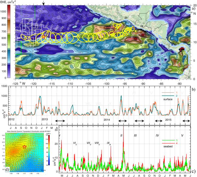
Figure 1 (a) The track of a mesoscale eddy (I) over 318 days from the coast towards the CCZ (licence areas shown with white and APEIs with green lines) and the BGR moorings site (star). Yellow lines encircle a local maximum (>80 cm) sea surface height (SSH) anomaly (AVISO31) at 10-day intervals. Colours reflect mean surface Eddy Kinetic Energy (EKE) over the period 2012.06.18-2013.05.01. (b) Timeseries of EKE at the sea-surface in the nearest () and the averaged over adjacent four grid points around the moorings site (). (c) EKE series in a layer 15–20 mab averaged over all three moorings () and at the northern site (). Here EKE = 0.5·(u′2 + v′2), and u′, v′ are the deviations of u,v velocities from the mean ū, v¯ averaged over the shown 3 and 2 years respectively. Eddies arrivals are indicated with black arrows and latin numbers I-V, IX (anticyclonic) and VIc-VIIIc (cyclonic). (d) Inset shows SSH anomaly (colours) and geostrophic currents (arrows) on the date of moorings deployment (2013.04.11). Figure was plotted using MATLAB R2015b (http://www.mathworks.com/).The map in this figure was queried from Google Static Map APIs (http://code.google.com/apis/maps/) using Get_google_map mapping package version 1.4 (https://uk.mathworks.com/matlabcentral/fileexchange/24113-get-google-map)
Figure 1 (a) The track of a mesoscale eddy (I) over 318 days from the coast towards the CCZ (licence areas shown with white and APEIs with green lines) and the BGR moorings site (star). Yellow lines encircle a local maximum (>80 cm) sea surface height (SSH) anomaly (AVISO31) at 10-day intervals. Colours reflect mean surface Eddy Kinetic Energy (EKE) over the period 2012.06.18-2013.05.01. (b) Timeseries of EKE at the sea-surface in the nearest () and the averaged over adjacent four grid points around the moorings site (). (c) EKE series in a layer 15–20 mab averaged over all three moorings () and at the northern site (). Here EKE = 0.5·(u′2 + v′2), and u′, v′ are the deviations of u,v velocities from the mean ū, v¯ averaged over the shown 3 and 2 years respectively. Eddies arrivals are indicated with black arrows and latin numbers I-V, IX (anticyclonic) and VIc-VIIIc (cyclonic). (d) Inset shows SSH anomaly (colours) and geostrophic currents (arrows) on the date of moorings deployment (2013.04.11). Figure was plotted using MATLAB R2015b (http://www.mathworks.com/).The map in this figure was queried from Google Static Map APIs (http://code.google.com/apis/maps/) using Get_google_map mapping package version 1.4 (https://uk.mathworks.com/matlabcentral/fileexchange/24113-get-google-map)CC BY · PubMed Central
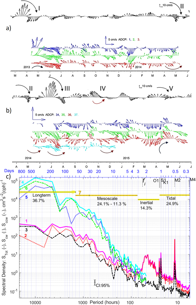
Figure 2 (a,b) Surface geostrophic velocity (AVISO31) (black) and residual currents at mooring No 1,2,3 (a), 34–36 (at the same sites) and 37 (b) shown in colours (3-daily averaged, layer 15–20 mab) for two deployment phases. The curved arrows indicate current veering during passage of eddies I-V. (c), Rotary spectral density estimates of seabed currents at mooring site 2 are shown with lines ,,3 for total, clockwise (cw) and counter-clockwise (ccw) components and similar lines ,, for the surface currents. Lomb-Scargle62,63 rotary spectra were calculated with unevenly sampled (1 and ¾ hours) data over the period 2013.04.11–2015.06.02. Confidence Intervals (CI = 95%) are included. Integration intervals over long-term, mesoscale, inertial, and tidal + high frequency internal wave’s bands and their contribution (%) in total spectra are shown with lines 7. High_Res_Figure_2 (https://figshare.com/s/78137cca3607d1266702). Figure was plotted using MATLAB R2015b (http://www.mathworks.com/).
Figure 2 (a,b) Surface geostrophic velocity (AVISO31) (black) and residual currents at mooring No 1,2,3 (a), 34–36 (at the same sites) and 37 (b) shown in colours (3-daily averaged, layer 15–20 mab) for two deployment phases. The curved arrows indicate current veering during passage of eddies I-V. (c), Rotary spectral density estimates of seabed currents at mooring site 2 are shown with lines ,,3 for total, clockwise (cw) and counter-clockwise (ccw) components and similar lines ,, for the surface currents. Lomb-Scargle62,63 rotary spectra were calculated with unevenly sampled (1 and ¾ hours) data over the period 2013.04.11–2015.06.02. Confidence Intervals (CI = 95%) are included. Integration intervals over long-term, mesoscale, inertial, and tidal + high frequency internal wave’s bands and their contribution (%) in total spectra are shown with lines 7. High_Res_Figure_2 (https://figshare.com/s/78137cca3607d1266702). Figure was plotted using MATLAB R2015b (http://www.mathworks.com/).CC BY · PubMed Central
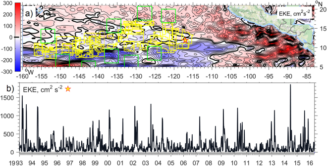
Figure 3 (a) The difference between the mean Eddy Kinetic Energy (EKE, defined as half of the horizontal velocity deviation from mean squared, isoline increment is 25 cm2∙s−2) of the altimetry–derived (AVISO31) ocean surface currents between the averaged eight El-Niño and seven La-Niña periods, calculated over 1993–2016. CCZ licence areas in the Tropical Pacific are shown with yellow and protected areas (APEIs) with green lines. (b) Surface EKE over the BGR mooring site (star on a map). High_Res_Figure_3 (https://figshare.com/s/2a1da19c8d6afe765e52). Figure was plotted using MATLAB R2015b (http://www.mathworks.com/).The map in this figure was queried from Google Static Map APIs (http://code.google.com/apis/maps/) using the Get_google_map mapping package version 1.4 (https://uk.mathworks.com/matlabcentral/fileexchange/24113-get-google-map).
Figure 3 (a) The difference between the mean Eddy Kinetic Energy (EKE, defined as half of the horizontal velocity deviation from mean squared, isoline increment is 25 cm2∙s−2) of the altimetry–derived (AVISO31) ocean surface currents between the averaged eight El-Niño and seven La-Niña periods, calculated over 1993–2016. CCZ licence areas in the Tropical Pacific are shown with yellow and protected areas (APEIs) with green lines. (b) Surface EKE over the BGR mooring site (star on a map). High_Res_Figure_3 (https://figshare.com/s/2a1da19c8d6afe765e52). Figure was plotted using MATLAB R2015b (http://www.mathworks.com/).The map in this figure was queried from Google Static Map APIs (http://code.google.com/apis/maps/) using the Get_google_map mapping package version 1.4 (https://uk.mathworks.com/matlabcentral/fileexchange/24113-get-google-map).CC BY · PubMed Central
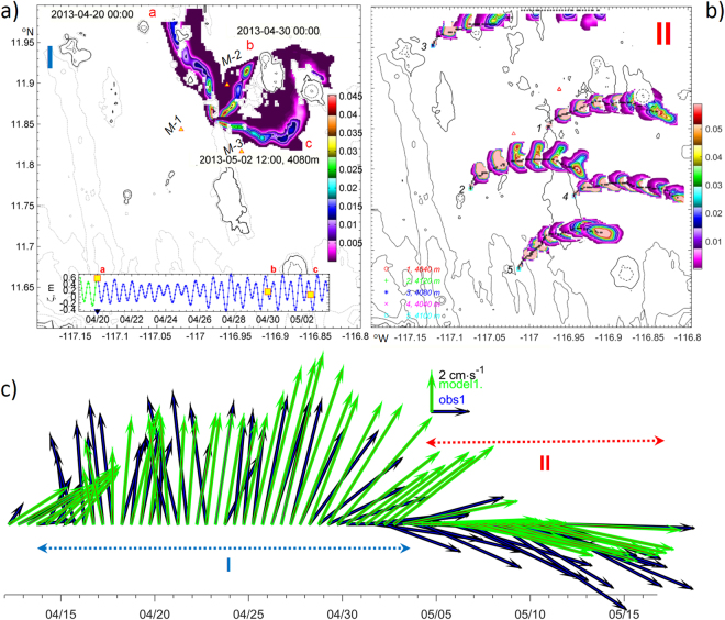
Figure 4 (a) Dissolved matter plume core tracks (colours, concentration in parts of unit), formed by neutral tracers released in period (April 2013) at three different dates (red ,,) marked on inset surface elevation (ζ, m) graph. Mooring sites are labelled with M-1, M-2 and M-3. (b) Plume core tracks formed by neutral tracers released in period from ‘calm’ sources (1,4,5) and two more energetic sites (2,3) adjacent to ‘hotspots’ (shown in 12-hour intervals). (c) Observed () and modelled () residual current vectors averaged over 12 hours at 20 mab at mooring site 1. High_Res_Fig. 4 (https://figshare.com/s/1cc75280276f0ead1508). Figure was plotted using MATLAB R2015b (http://www.mathworks.com/).
Figure 4 (a) Dissolved matter plume core tracks (colours, concentration in parts of unit), formed by neutral tracers released in period (April 2013) at three different dates (red ,,) marked on inset surface elevation (ζ, m) graph. Mooring sites are labelled with M-1, M-2 and M-3. (b) Plume core tracks formed by neutral tracers released in period from ‘calm’ sources (1,4,5) and two more energetic sites (2,3) adjacent to ‘hotspots’ (shown in 12-hour intervals). (c) Observed () and modelled () residual current vectors averaged over 12 hours at 20 mab at mooring site 1. High_Res_Fig. 4 (https://figshare.com/s/1cc75280276f0ead1508). Figure was plotted using MATLAB R2015b (http://www.mathworks.com/).CC BY · PubMed Central
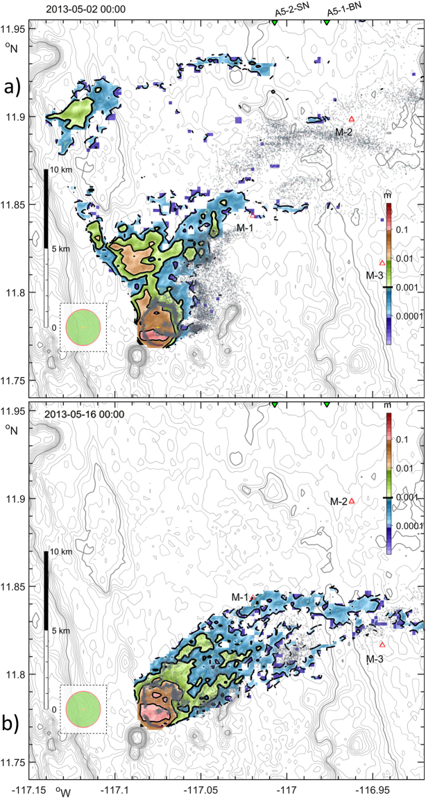
Figure 5 (a) Model particulate plume on the 10th day after start release (at the end of eddy passing period) containing 5.7·105 individual particles suspended in a water (grey dots) and settled on seafloor (colours). The area with substantial accumulated sediment layer thickness (in m) is shown over bathymetry (grey lines, 50 m). Points along the nodule collector tracks were aligned with equally-spaced Archimedes spiral, and shown on a dashed in-cut to indicate the scale of the harvested zone during the last day (red) and since the beginning of experiment (green). Red and green triangles indicate three mooring sites, labelled with M-1, M-2 and M-3, and two sediment core sampling sites53 respectively. (b), Settling footprint after 10 days of a similar SPM release over period without eddy impact. High_Res_Fig. 5 (https://figshare.com/s/5472457ce071bd654305) and animations are available on-line via Supplementary Info Media3_2D_plume_movie.gif (https://figshare.com/s/abd96d10a22263c42e3b). Figure and media animation were plotted using MATLAB R2015b (http://www.mathworks.com/).
Figure 5 (a) Model particulate plume on the 10th day after start release (at the end of eddy passing period) containing 5.7·105 individual particles suspended in a water (grey dots) and settled on seafloor (colours). The area with substantial accumulated sediment layer thickness (in m) is shown over bathymetry (grey lines, 50 m). Points along the nodule collector tracks were aligned with equally-spaced Archimedes spiral, and shown on a dashed in-cut to indicate the scale of the harvested zone during the last day (red) and since the beginning of experiment (green). Red and green triangles indicate three mooring sites, labelled with M-1, M-2 and M-3, and two sediment core sampling sites53 respectively. (b), Settling footprint after 10 days of a similar SPM release over period without eddy impact. High_Res_Fig. 5 (https://figshare.com/s/5472457ce071bd654305) and animations are available on-line via Supplementary Info Media3_2D_plume_movie.gif (https://figshare.com/s/abd96d10a22263c42e3b). Figure and media animation were plotted using MATLAB R2015b (http://www.mathworks.com/).CC BY · PubMed Central
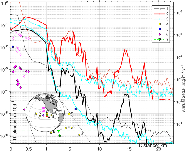
Figure 6 Settled sediment thickness (m) as a function of distance from the source are shown with 1 black (averaged) and red (maximum) lines computed in numerical Experiments III under eddy impact using two vertical mixing schemes: KL1068 (bold) and PP8167 (thin). Cyan lines show the averaged (solid) and maximum (dashed) thickness of sediments settled during the other 10 days of SPM release, when the impact of the eddy vanished. Yellow symbols 4 show JGOFS77–80 sediment trap rates and their location in Eastern Pacific. Symbols , show visual and measured data from 15 sediment traps collected in BIE50,51, while empty diamonds show BIE trap values scaled by suspended mass ratio R = 31.8 over 10 days between this numerical experiment (454,756t) and in-situ BIE trials (1,427t of sediments were dispersed during 19 days at a rate of 4.2 kg·s−1 by a six-meter-wide “benthic disturber” that was towed in 49 parallel rows within a 3300 m × 150 m polygon)51. Green line 7 indicates the natural sedimentation rate at two A5 stations53. High_Res_Fig. 6 (https://figshare.com/s/d984083a59832f4227ea) and Table 3 are available on-line via Supplementary Info. Figure was plotted using MATLAB R2015b (http://www.mathworks.com). The map in this figure was generated by MATLAB R2015b with M_Map (a mapping package, http://www.eos.ubc.ca/~rich/map.html).
Figure 6 Settled sediment thickness (m) as a function of distance from the source are shown with 1 black (averaged) and red (maximum) lines computed in numerical Experiments III under eddy impact using two vertical mixing schemes: KL1068 (bold) and PP8167 (thin). Cyan lines show the averaged (solid) and maximum (dashed) thickness of sediments settled during the other 10 days of SPM release, when the impact of the eddy vanished. Yellow symbols 4 show JGOFS77–80 sediment trap rates and their location in Eastern Pacific. Symbols , show visual and measured data from 15 sediment traps collected in BIE50,51, while empty diamonds show BIE trap values scaled by suspended mass ratio R = 31.8 over 10 days between this numerical experiment (454,756t) and in-situ BIE trials (1,427t of sediments were dispersed during 19 days at a rate of 4.2 kg·s−1 by a six-meter-wide “benthic disturber” that was towed in 49 parallel rows within a 3300 m × 150 m polygon)51. Green line 7 indicates the natural sedimentation rate at two A5 stations53. High_Res_Fig. 6 (https://figshare.com/s/d984083a59832f4227ea) and Table 3 are available on-line via Supplementary Info. Figure was plotted using MATLAB R2015b (http://www.mathworks.com). The map in this figure was generated by MATLAB R2015b with M_Map (a mapping package, http://www.eos.ubc.ca/~rich/map.html).CC BY · PubMed Central

Verification

Claims the paper makes

The claims and statistics of this paper haven’t been checked yet.

Run the check — free, no account needed. It reads the open-access text and checks the sources it cites.

A few free checks a day · papers already verified open instantly · results are public

Claims other papers make about this one

Each is checked against this paper’s own text: does it say what the citing paper says it does?

Self-check

Percentages, sums and reported differences re-computed from the paper’s own numbers.

The self-check needs the paper’s full text.

Citations

Cites

Show all 76 references

Research works printed but not linked: 3

  1. Thiel, H., Foell, E. J. & Schriever, G. Potential environmental effects of deep seabed mining. Berichte aus dem Zentrum für Meeres- und Klimaforschung der Universität Hamburg 26, 243 (1991).
  2. Zyryanov, V. N. Topographic eddies in a stratified ocean. Regular and Chaotic Dynamics 11, 491–521, https://doi.org/10.1070/RD2006v011n04ABEH000367 (2006). · DOI
  3. Roe, P. L. Some contributions to the modelling of discontinuous flows, in Large-scale computations in fluid mechanics; Proceedings of the Fifteenth Summer Seminar on Applied Mathematics, 1983. (eds Lee, R. L. Sani, R. L. Shih, T. M. & Gresho, P. M.), 2, 163–193 (American Mathematical Society, 1985).

Cited by

Sorted by citations

See all 131

Metadata

Authors
Aleynik, D., Inall, M. E., Dale, A., & Vink, A.
Affiliations
Scottish Association For Marine Science (GB)
Corresponding author
Aleynik, Dmitry
Venue
Scientific Reports
Published
2017-12-05
Volume
7
Issue
1
Pages
16959-16959
ISSN
2045-2322 (ISSN-L)
OpenAlex
W2770479302
Cited by
131
References
76
Citations by year
2026: 12 · 2025: 14 · 2024: 22 · 2023: 11 · 2022: 28 · 2021: 8 · 2020: 14 · 2019: 15 · 2018: 7
FWCI
6.55
Type
journal article
Language
en
Open access
Locations
  • Scientific Reports (publishedVersion, cc-by)
  • Europe PMC (PubMed Central) (publishedVersion, cc-by)
  • PubMed Central (publishedVersion, cc-by)
  • PubMed (publishedVersion)
  • DOAJ (DOAJ: Directory of Open Access Journals) (submittedVersion)
  • Zenodo (CERN European Organization for Nuclear Research) (submittedVersion, cc-by)
Funders
  • European Commission (603418)
  • Natural Environment Research Council
Topics
  • Physical Sciences › Earth and Planetary Sciences › Oceanography › Oceanographic and Atmospheric Processes
  • Physical Sciences › Earth and Planetary Sciences › Oceanography › Marine Biology and Ecology Research
  • Physical Sciences › Earth and Planetary Sciences › Oceanography › Marine Plankton and Biogeochemistry
Keywords
polymetallic nodule mining, deep-sea mining, sediment plumes, mesoscale eddies, abyssal currents, tidal forcing, suspended sediment resuspension, plume dispersion, central tropical Pacific, deep-sea mining impacts

About these checks

Registry, retraction, Cites and statistics results are computed, not judged, with one exception: a printed reference that no index lists is read once by a model before it counts as a citation error. Claims are extracted by a model and kept only when their quote appears verbatim in the text; each cited source is then checked, with a model’s help, for whether it says what the claim relies on. Those verdicts can be wrong — read the claim’s quote and the cited source before relying on one.

Statistics and arithmetic are recomputed, not judged.

Confidence bands are shown only for fields calibrated on our annotated test set. None is calibrated yet, so no band is shown.

What counts as a claim ›How we measure confidence ›How we check this ›

Are you an author, or do you see a problem with this page? Request a review