Cited by 143

The DOI matches its Crossref record.

There is More than a Power Law in Zipf

Cristelli, Matthieu, Batty, Michael, Pietronero, Luciano·2012·Scientific Reports

Overview

The claims and statistics of this paper haven’t been checked yet.

Run the check — free, no account needed. It reads the open-access text and checks the sources it cites.

A few free checks a day · papers already verified open instantly · results are public

Integrity signals

Registry

Crossref · 10.1038/srep00812

Cites

Statistics

Figures

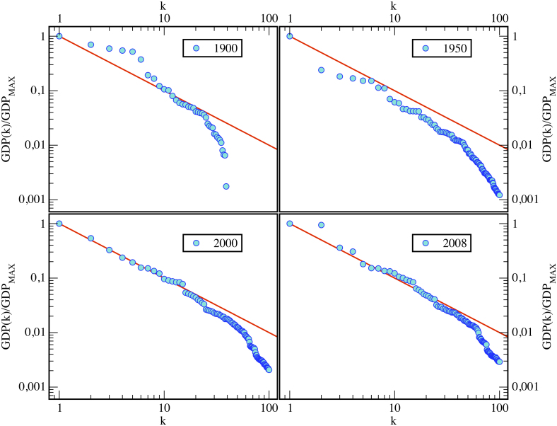
Figure 1 Zipf’s Law for National Gross Domestic Products 1900-2008. The Gross Domestic Products of nations appear to show a more and more a Zipfian behavior over the last one hundred years. We propose a fascinating interpretation of this evidence in terms of globalization. In fact we have said that a set is Zipfian if there exists an internal coherence among its elements. As the world has become more fully globalized, we observe that Zipf’s Law holds for an increasing number for countries. In fact in 2000 and 2008 we observe that not only the highest GDPs satisfy Zipf’s Law (red line) but also the top fifty economies and that the rank at which the deviation from a Zipf’s Law behavior starts increases in time, suggesting the idea that world economic system is getting more and more coherent, i.e. globalized. Globalization is making the world fully coherent/integrated with respect to the richness distribution among its units (i.e. countries) while this degree of integration has not yet been reached by the world’s national populations (see Fig. 3). Sources: Wikipedia: various pages on GDP http://en.wikipedia.org/wiki/List_of_countries_by_GDP_(nominal) and http://en.wikipedia.org/wiki/List_of_regions_by_past_GDP_(PPP).
Figure 1 Zipf’s Law for National Gross Domestic Products 1900-2008. The Gross Domestic Products of nations appear to show a more and more a Zipfian behavior over the last one hundred years. We propose a fascinating interpretation of this evidence in terms of globalization. In fact we have said that a set is Zipfian if there exists an internal coherence among its elements. As the world has become more fully globalized, we observe that Zipf’s Law holds for an increasing number for countries. In fact in 2000 and 2008 we observe that not only the highest GDPs satisfy Zipf’s Law (red line) but also the top fifty economies and that the rank at which the deviation from a Zipf’s Law behavior starts increases in time, suggesting the idea that world economic system is getting more and more coherent, i.e. globalized. Globalization is making the world fully coherent/integrated with respect to the richness distribution among its units (i.e. countries) while this degree of integration has not yet been reached by the world’s national populations (see Fig. 3). Sources: Wikipedia: various pages on GDP http://en.wikipedia.org/wiki/List_of_countries_by_GDP_(nominal) and http://en.wikipedia.org/wiki/List_of_regions_by_past_GDP_(PPP).CC BY-NC-ND · PubMed Central
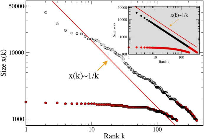
Figure 2 Zipf’s Law for the Richest Billionaires in the United States. The richest 390 persons in the US are billionaires whose wealth we plot against their rank as the uppermost set of points (the first 195 richest being grey circles, the second 195 poorest being red circles). The second set is the sub-sample that we translate to the original ranks and plot as the set of red circle points below the diagonal straight line which is the pure Zipf plot associated with . The inset is a pure Zipf plot dimensioned to the entire set of 390 billionaires and the poorest sub-sample of 195. (Source: Forbes List http://www.forbes.com/).
Figure 2 Zipf’s Law for the Richest Billionaires in the United States. The richest 390 persons in the US are billionaires whose wealth we plot against their rank as the uppermost set of points (the first 195 richest being grey circles, the second 195 poorest being red circles). The second set is the sub-sample that we translate to the original ranks and plot as the set of red circle points below the diagonal straight line which is the pure Zipf plot associated with . The inset is a pure Zipf plot dimensioned to the entire set of 390 billionaires and the poorest sub-sample of 195. (Source: Forbes List http://www.forbes.com/).CC BY-NC-ND · PubMed Central
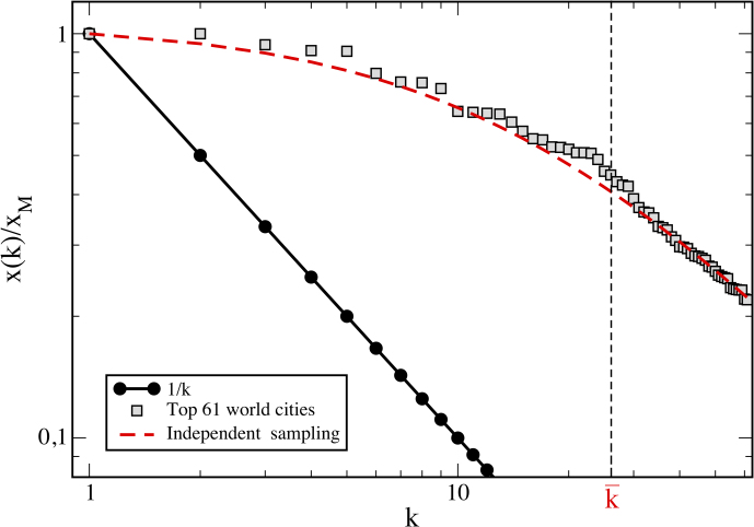
Figure 3 Rank Size of World Cities and Deviation from Zipf’s Law. The top 61 ‘world cities proper’ normalized as plotted in the grey squares are used to compute the modified rank size equation Eq.(3) – dashed red line – compared to the pure rank size equation which is the solid black line. Note the value of , below which values do not accord to Zipf’s Law in contrast to those above. The data is from the compilation of 65 separate databases (Sources: Wikipedia http://en.wikipedia.org/wiki/List_of_cities_proper_by_population).
Figure 3 Rank Size of World Cities and Deviation from Zipf’s Law. The top 61 ‘world cities proper’ normalized as plotted in the grey squares are used to compute the modified rank size equation Eq.(3) – dashed red line – compared to the pure rank size equation which is the solid black line. Note the value of , below which values do not accord to Zipf’s Law in contrast to those above. The data is from the compilation of 65 separate databases (Sources: Wikipedia http://en.wikipedia.org/wiki/List_of_cities_proper_by_population).CC BY-NC-ND · PubMed Central
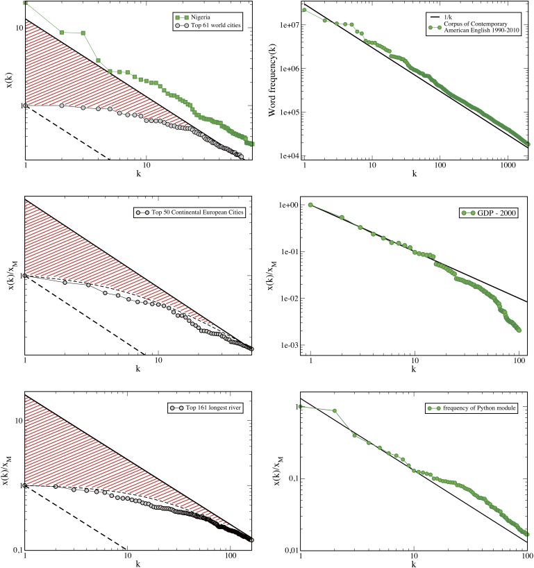
Figure 4 Rank-Size Laws Illustrating Different Degrees of Coherence. Top Left: Rank-size for the largest world cities showing the absence of truly global cities which have developed in relation to all other cities. Therefore the world is not a coherent/fully integrated system and represents the wrong scale at which city size samples must be aggregated to obtain a Zipf’s Law. Instead Nigeria (green solid line) shows a nearly perfect Zipfian behavior. Nigeria which is separate from the rest of Africa, represents a city system which has developed more uniformly in a more integrated fashion, The Nigeria rank size law has been rescaled for clarity; Centre Left: Rank-size of the fifty largest European continental cities (i.e. the European part of Russia and UK are excluded). As in the case of the world cities, we observe absence of coherence at this geographical scale; Bottom Left: River formations are mainly due to geographical and morphological constraints on the Earth’s surface. Hence a Zipf’s Law is not expected and in fact the river rank size rule is well approximated by the curve (dashed black line), predicted by an independent sampling procedure without any screening effect; Top Right: For the frequency of words in the Corpus of Contemporary American English, a quasi-perfect Zipf’s Law is observed over the 2000 (and more) most used words. Linguistic systems are fully coherent with respect to our interpretation of Zipf’s Law. Centre Right: If we rank the Gross Domestic Product (GDP) of world countries, we observe a Zipfian behavior for the 30 richest. Bottom Right: As for words, a Zipf’s Law also appears in the frequency of usage of Python modules in a computer science project domain. Sources: Nigeria from the Mathematica database see Fig. 5; the top 61 country populations is from Wikipedia, see Fig. 2; the top 50 continental European city populations from http://www.citymayors.com/features/euro_cities.html; the top 161 river lengths from Wikipedia http://en.wikipedia.org/wiki/ List_of_rivers_by_length; top 2000 COCA words from http://corpus.byu.edu/coca/; GDP from Wikipedia http://en.wikipedia.org/wiki/List_of_countries_by_GDP_(nominal); the frequency of Python module usage from http://www.algorithm.co.il/blogs/math/python-module-usage-statistics/
Figure 4 Rank-Size Laws Illustrating Different Degrees of Coherence. Top Left: Rank-size for the largest world cities showing the absence of truly global cities which have developed in relation to all other cities. Therefore the world is not a coherent/fully integrated system and represents the wrong scale at which city size samples must be aggregated to obtain a Zipf’s Law. Instead Nigeria (green solid line) shows a nearly perfect Zipfian behavior. Nigeria which is separate from the rest of Africa, represents a city system which has developed more uniformly in a more integrated fashion, The Nigeria rank size law has been rescaled for clarity; Centre Left: Rank-size of the fifty largest European continental cities (i.e. the European part of Russia and UK are excluded). As in the case of the world cities, we observe absence of coherence at this geographical scale; Bottom Left: River formations are mainly due to geographical and morphological constraints on the Earth’s surface. Hence a Zipf’s Law is not expected and in fact the river rank size rule is well approximated by the curve (dashed black line), predicted by an independent sampling procedure without any screening effect; Top Right: For the frequency of words in the Corpus of Contemporary American English, a quasi-perfect Zipf’s Law is observed over the 2000 (and more) most used words. Linguistic systems are fully coherent with respect to our interpretation of Zipf’s Law. Centre Right: If we rank the Gross Domestic Product (GDP) of world countries, we observe a Zipfian behavior for the 30 richest. Bottom Right: As for words, a Zipf’s Law also appears in the frequency of usage of Python modules in a computer science project domain. Sources: Nigeria from the Mathematica database see Fig. 5; the top 61 country populations is from Wikipedia, see Fig. 2; the top 50 continental European city populations from http://www.citymayors.com/features/euro_cities.html; the top 161 river lengths from Wikipedia http://en.wikipedia.org/wiki/ List_of_rivers_by_length; top 2000 COCA words from http://corpus.byu.edu/coca/; GDP from Wikipedia http://en.wikipedia.org/wiki/List_of_countries_by_GDP_(nominal); the frequency of Python module usage from http://www.algorithm.co.il/blogs/math/python-module-usage-statistics/CC BY-NC-ND · PubMed Central
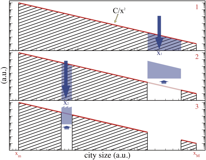
Figure 5 Successive Conditioned Draws. When we extract an object (or a city size) such as x1, we remove a section (blue slice in panel 1) of the probability density around the drawn value. See the text for the details of how to compute the slice to remove (Eq.7). Then the density moves to the reduced distribution in panel 2 from which the next object is drawn in the same way with the slice associated with x2 being removed in panel 3.
Figure 5 Successive Conditioned Draws. When we extract an object (or a city size) such as x1, we remove a section (blue slice in panel 1) of the probability density around the drawn value. See the text for the details of how to compute the slice to remove (Eq.7). Then the density moves to the reduced distribution in panel 2 from which the next object is drawn in the same way with the slice associated with x2 being removed in panel 3.CC BY-NC-ND · PubMed Central
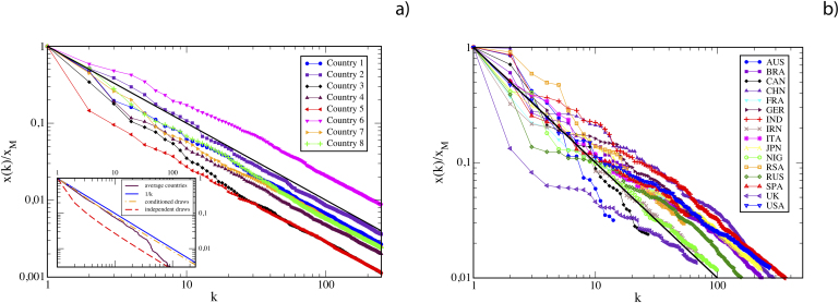
Figure 6 Real (Zipfian) and Sampled Theoretical Rank-Size Law. Left (a): Eight sets of samples of 250 cities each drawn using the random conditioning algorithm explained in the text, rescaled in order to have the same maximum value and compared with a pure Zipf’s Law (black solid line). In the inset, we report the average rank-size law (dashed orange line) of 200 simulated countries from which the eight reported in the main box are extracted. We compare this with the rank-size rule produced by independent random samplings (red dashed line) and with the average over the 16 countries of panel b) (maroon solid line). We observe that the conditioned sampling algorithm produces a striking result very close to a pure Zipf ‘s Law (blue solid line). Right (b): Rank-size rules for the cities in 16 world countries collapsed in order to have the same maximum values and comparable with Zipf’s Law for the same (black solid line) (Source: Wolfram Mathematica online database).
Figure 6 Real (Zipfian) and Sampled Theoretical Rank-Size Law. Left (a): Eight sets of samples of 250 cities each drawn using the random conditioning algorithm explained in the text, rescaled in order to have the same maximum value and compared with a pure Zipf’s Law (black solid line). In the inset, we report the average rank-size law (dashed orange line) of 200 simulated countries from which the eight reported in the main box are extracted. We compare this with the rank-size rule produced by independent random samplings (red dashed line) and with the average over the 16 countries of panel b) (maroon solid line). We observe that the conditioned sampling algorithm produces a striking result very close to a pure Zipf ‘s Law (blue solid line). Right (b): Rank-size rules for the cities in 16 world countries collapsed in order to have the same maximum values and comparable with Zipf’s Law for the same (black solid line) (Source: Wolfram Mathematica online database).CC BY-NC-ND · PubMed Central

Verification

Claims the paper makes

The claims and statistics of this paper haven’t been checked yet.

Run the check — free, no account needed. It reads the open-access text and checks the sources it cites.

A few free checks a day · papers already verified open instantly · results are public

Claims other papers make about this one

Each is checked against this paper’s own text: does it say what the citing paper says it does?

Self-check

Percentages, sums and reported differences re-computed from the paper’s own numbers.

The self-check needs the paper’s full text.

Citations

Cites

No references could be resolved yet.

Research works printed but not linked: 20

  1. Zipf, G. K. Human behavior and the principle of least effort (Addison-Wesley, Cambridge, MA, 1949).
  2. Saichev, A., Malevergne, Y. & Sornette, D. Theory of Zipf’s law and beyond (Lecture Notes in Economics and Mathematical Systems 632, Springer, Heidelberg, Germany, 2010). · DOI
  3. Clauset, A., Shalizi, C. R., & Newman, M. E. J. Power-law distributions in empirical data. SIAM Review 51, 661–703 (2009). · DOI · Paper page
  4. Blank, A. & Solomon, S. Power laws in cities population, financial markets and internet sites: Scaling and systems with a variable number of components. Physica A 287, 279–288 (2000). · DOI
  5. Lotka, A. J. The frequency distribution of scientific production. Journal of the Washington Academy of Sciences 16, 317–323 (1926).
  6. Gabaix, X. Zipf’s law for cities: An explanation. Quarterly Journal of Economics 114, 739–767 (1999). · DOI
  7. Axtell, R. L. Zipf distribution of U.S. firm sizes. Science 293, 1818–1820 (2001). · DOI · Paper page
  8. Barabási, A.-L. & Albert, R. Emergence of scaling in random networks. Science 286. 509–512 (1999). · DOI · Paper page
  9. Barabási, A.-L. The origin of bursts and heavy tails in human dynamics. Nature 435, 207–211 (2005). · DOI · Paper page
  10. Perline, R. Strong, weak and false inverse power laws. Statistical Science 20, 68–88 (2005). · DOI
  11. Montroll, E. W. & Schlesinger, M. F. On 1/f noise and other distributions with long tails. Proceedings of the National Academy of Sciences USA 79, 3380–3383 (1982). · DOI
  12. Krugman, P. The great illusion, The New York Times, August 15, A17 (2008), available at http://www.nytimes.com/2008/08/15/opinion/15krugman.html?_r=0 accessed 5/10/2012.
  13. Eeckhout, J. Gibrat’s law for (all) cities. American Economic Review 94, 1429–1451 (2005). · DOI
  14. Rose, A. K. Cities and countries. Journal of Money, Credit and Banking 38, 2225–2245 (2006). · DOI
  15. Pietronero, L., Tosatti, E., Tosatti, V. & Vespignani, A. Explaining the uneven distribution of numbers in nature: the laws of Benford and Zipf. Physica A 293, 297–304 (2001). · DOI
  16. Sassen, S. The global city: New York, London, Tokyo (Princeton University Press, Princeton, NJ, 2001). · DOI
  17. Rosen, K. T. & Resnick, M. The size distribution of cities: An examination of the Pareto law and primacy. Journal of Urban Economics 8, 165–186 (1980). · DOI
  18. Soo, K. T. Zipf's law for cities: A cross country investigation. Regional Science and Urban Economics 35, 239–263 (2005). · DOI
  19. Cheshire, P. Trends in sizes and structure of urban areas. Handbook of Regional and Urban Economics, 3, 1339–1373 (1999). · DOI
  20. Stanley, M. H. R., Buldyrev, S. V., Havlin, S., Mantegna, R. N., Salinger, M. A. & Stanley, H. E. Zipf plots and the size distribution of firms. Economics Letters 49, 453–457 (1995). · DOI

Cited by

Sorted by citations

Metadata

Authors
Cristelli, M., Batty, M., & Pietronero, L.
Venue
Scientific Reports
Published
2012-11-08
Volume
2
Issue
1
ISSN
2045-2322
Cited by
143
References
0
Language
en

About these checks

Registry, retraction, Cites and statistics results are computed, not judged, with one exception: a printed reference that no index lists is read once by a model before it counts as a citation error. Claims are extracted by a model and kept only when their quote appears verbatim in the text; each cited source is then checked, with a model’s help, for whether it says what the claim relies on. Those verdicts can be wrong — read the claim’s quote and the cited source before relying on one.

Statistics and arithmetic are recomputed, not judged.

Confidence bands are shown only for fields calibrated on our annotated test set. None is calibrated yet, so no band is shown.

What counts as a claim ›How we measure confidence ›How we check this ›

Are you an author, or do you see a problem with this page? Request a review