

The DOI matches its Crossref record; 4 of the 4 references it cites were found in a registry or an index.
Deep learning for automated size and shape analysis of nanoparticles in scanning electron microscopy
Abstract
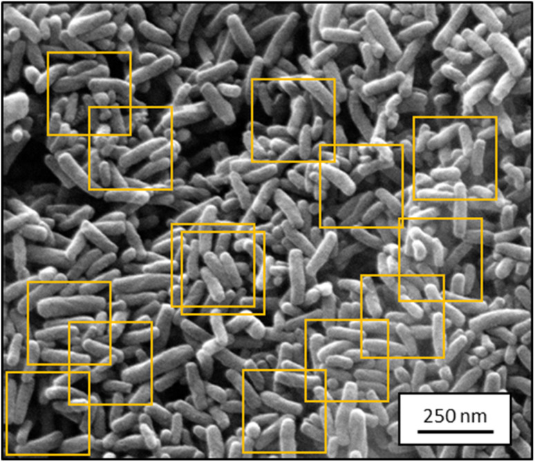
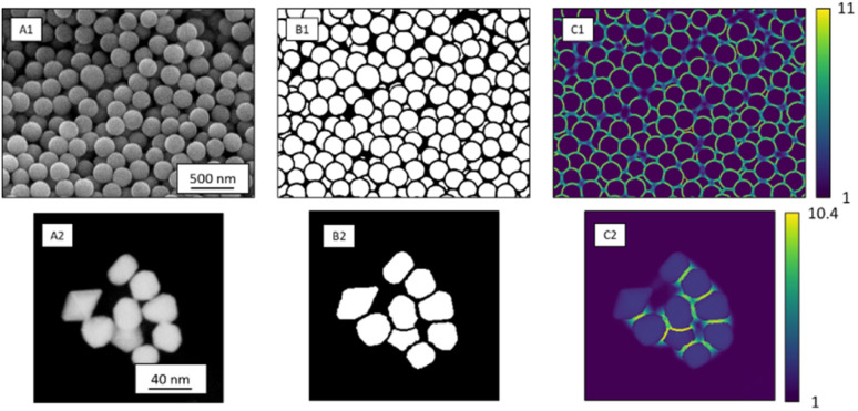
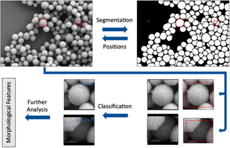
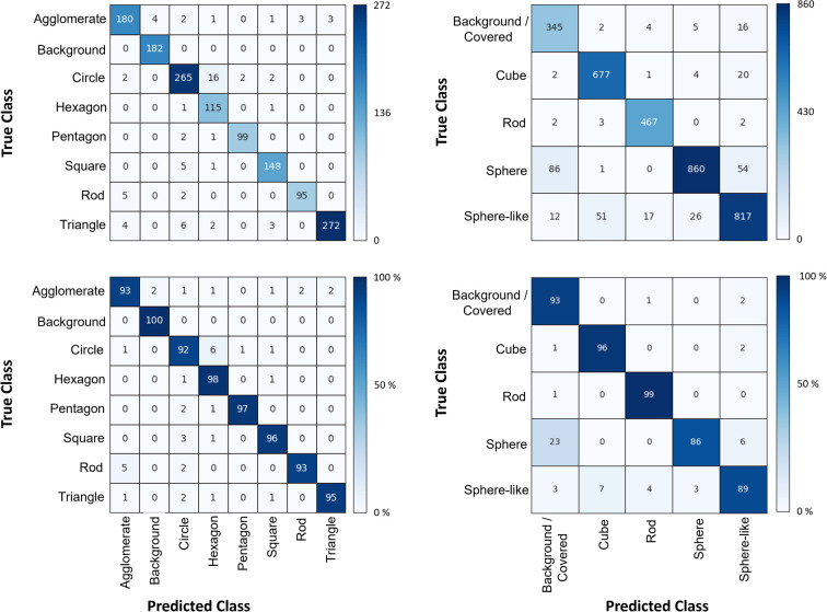
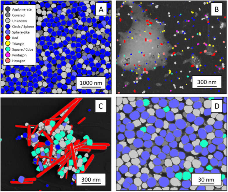
Particles depicted in scanning electron micrographs are automatically identified and classified according to size and shape with a deep-learning algorithm. The procedure works for both SE images and STEM images.
Overview
The claims and statistics of this paper haven’t been checked yet.
Run the check — free, no account needed. It reads the open-access text and checks the sources it cites.
Integrity signals
Registry
Cites
Statistics
Figures
Verification
Claims the paper makes
The claims and statistics of this paper haven’t been checked yet.
Run the check — free, no account needed. It reads the open-access text and checks the sources it cites.
Claims other papers make about this one
Each is checked against this paper’s own text: does it say what the citing paper says it does?
In the citing paper
“Deep-learning procedures based on convolutional neural networks have already been utilized to automate the SEM image analysis. However, such solutions have been practiced mostly in the context of material sciences.61-64”
From SEMTWIST Quantification of Biofilm Infection in Human Chronic Wound Using Scanning Electron Microscopy and Machine Learning (2025) · cites this paper as [62]
Self-check
Percentages, sums and reported differences re-computed from the paper’s own numbers.
The self-check needs the paper’s full text.
Citations
Cites
U-Net: Convolutional Networks for Biomedical Image Segmentation
Ronneberger, O., Fischer, P., & Brox, T. (2015) · Lecture notes in computer science · doi:10.1007/978-3-319-24574-4_28 · Cited by 99,404
LeCun, Y., Bengio, Y., & Hinton, G. (2015) · Nature · doi:10.1038/nature14539 · Cited by 84,126
Deep Residual Learning for Image Recognition
He, K., Zhang, X., Ren, S., & Sun, J. (2015) · arXiv · doi:10.48550/arxiv.1512.03385 · Cited by 4,196
Recent advances and applications of deep learning methods in materials science
Choudhary, K., DeCost, B., Chen, C., Jain, A., Tavazza, F., Cohn, R., Park, C. W., Choudhary, A., Agrawal, A., Billinge, S. J. L., et al. (2022) · npj Computational Materials · doi:10.1038/s41524-022-00734-6 · Cited by 1,172
Research works printed but not linked: 32
- Fissan, 2014, Anal. Methods, 6, 7324, 10.1039/C4AY01203H · DOI
- Modena, 2019, Adv. Mater., 31, 1901556, 10.1002/adma.201901556 · DOI
- Bals, 2022, Materialwiss. Werkstofftech., 53, 270, 10.1002/mawe.202100285 · DOI
- Modarres, 2017, Sci. Rep., 7, 13282, 10.1038/s41598-017-13565-z · DOI
- Holm, 2020, Metall. Mater. Trans. A, 51, 5985, 10.1007/s11661-020-06008-4 · DOI
- Schmidt, 2019, npj Comput. Mater., 5, 83, 10.1038/s41524-019-0221-0 · DOI
- Timoshenko, 2018, Nano Lett., 19, 520, 10.1021/acs.nanolett.8b04461 · DOI
- Oktay, 2019, Micron, 120, 113, 10.1016/j.micron.2019.02.009 · DOI
- Ede, 2020, Sci. Rep., 10, 8332, 10.1038/s41598-020-65261-0 · DOI
- Ilett, 2020, J. Microsc., 279, 177, 10.1111/jmi.12853 · DOI
- Kim, 2020, Nanoscale, 12, 19461, 10.1039/D0NR04140H · DOI
- Lee, 2020, ACS Nano, 14, 17125, 10.1021/acsnano.0c06809 · DOI
- A.Krizhevsky , I.Sutskever and G. E.Hinton , Presented in part at the Proceedings of the 25th International Conference on Neural Information Processing Systems – Volume 1 , Lake Tahoe , Nevada , 2012
- K.He , X.Zhang , S.Ren and J.Sun , Presented in part at the 2016 IEEE Conference on Computer Vision and Pattern Recognition (CVPR), 27–30 June 2016 , 2016
- Jacobs, 2022, Comput. Mater. Sci., 211, 111527, 10.1016/j.commatsci.2022.111527 · DOI
- Treder, 2022, Microscopy, 71, i100, 10.1093/jmicro/dfab043 · DOI
- I.Goodfellow , Y.Bengio and A.Courville , Deep Learning , MIT Press , 2016
- Z.Zhou , M. M.Rahman Siddiquee , N.Tajbakhsh and J.Liang , in Deep Learning in Medical Image Analysis and Multimodal Learning for Clinical Decision Support , Springer , 2018 , pp. 3–11 , 10.1007/978-3-030-00889-5_1 · DOI
- Ruehle, 2021, Sci. Rep., 11, 4942, 10.1038/s41598-021-84287-6 · DOI
- Zhou, 2020, IEEE Trans. Med. Imag., 39, 1856, 10.1109/TMI.2019.2959609 · DOI
- G.Huang , Z.Liu , L.van der Maaten and K. Q.Weinberger , Presented in part at the 2017 IEEE Conference on Computer Vision and Pattern Recognition ( CVPR ), 2017 , pp. 21–26
- Unnikrishnan, 2007, IEEE Trans. Pattern Anal. Mach. Intell., 29, 929, 10.1109/TPAMI.2007.1046 · DOI
- Saaim, 2022, Ultramicroscopy, 233, 113437, 10.1016/j.ultramic.2021.113437 · DOI
- D. P.Kingma and J.Ba , arXiv , 2015 , preprint, arXiv:1412.6980, 10.48550/arXiv.1412.6980 · DOI · Paper page
- M.Abadi , P.Barham , J.Chen , Z.Chen , A.Davis , J.Dean , M.Devin , S.Ghemawat , G.Irving , M.Isard , M.Kudlur , J.Levenberg , R.Monga , S.Moore , D. G.Murray , B.Steiner , P.Tucker , V.Vasudevan , P.Warden , M.Wicke , Y.Yu and X.Zheng , Presented in Part at the 12th USENIX Symposium on Operating Systems Design and Implementation (OSDI 16) , Savannah, GA, USA , 2016
- Aldrich, 1997, Stat. Sci., 12, 162, 10.1214/ss/1030037906 · DOI
- K.He , X.Zhang , S.Ren and J.Sun , arXiv , 2015 , preprint, arXiv:1502.01852, 10.48550/arXiv.1502.01852 · DOI
- M. D.Zeiler and R.Fergus , Presented in Part at the Computer Vision – ECCV 2014 , Cham , 2014
- Munoz-Marmol, 2015, Nanomedicine, 11, 457, 10.1016/j.nano.2014.07.006 · DOI
- Hughes, 2015, PeerJ, 2, e671v671
- Baiyasi, 2020, J. Phys. Chem. A, 124, 5262, 10.1021/acs.jpca.0c03190 · DOI
- De Siqueira, 2014, Microsc. Res. Tech., 77, 71, 10.1002/jemt.22314 · DOI
Cited by
Sorted by citations
Singh, S., Muniz De Oliveira, F., Wang, C., Kumar, M., Xuan, Y., DeMazumder, D., Sen, C. K., & Roy, S. (2025) · Advances in Wound Care · doi:10.1089/wound.2024.0291 · Cited by 6
Metadata
- Authors
- Bals, J., & Epple, M.
- Venue
- RSC Advances
- Publisher
- Royal Society of Chemistry (RSC)
- Published
- 2023
- Volume
- 13
- Issue
- 5
- Pages
- 2795-2802
- ISSN
- 2046-2069
- PMC
- PMC9850277
- Cited by
- 93
- References
- 4
- Language
- en
About these checks
Registry, retraction, Cites and statistics results are computed, not judged, with one exception: a printed reference that no index lists is read once by a model before it counts as a citation error. Claims are extracted by a model and kept only when their quote appears verbatim in the text; each cited source is then checked, with a model’s help, for whether it says what the claim relies on. Those verdicts can be wrong — read the claim’s quote and the cited source before relying on one.
Statistics and arithmetic are recomputed, not judged.
Confidence bands are shown only for fields calibrated on our annotated test set. None is calibrated yet, so no band is shown.
What counts as a claim ›How we measure confidence ›How we check this ›
Are you an author, or do you see a problem with this page? Request a review
