

The DOI matches its Crossref record; 61 of the 61 references it cites were found in a registry or an index; none of the 55 sources its claims cite is checked for support yet.
Taming Thiemann’s Hamiltonian constraint in canonical loop quantum gravity: Reversibility, eigenstates, and graph-change analysis
Open accessPublished version of a preprint
Abstract
The Hamiltonian constraint remains an elusive object in loop quantum gravity because its action on spinnetworks leads to changes in their corresponding graphs. As a result, calculations in loop quantum gravity are often considered unpractical, and neither the eigenstates of the Hamiltonian constraint, which form the physical space of states, nor the concrete effect of its graph-changing character on observables are entirely known. Much worse, there is no reference value to judge whether the commonly adopted graph-preserving approximations lead to results anywhere close to the non-approximated dynamics. Our work sheds light on many of these issues, by devising a new numerical tool that allows us to implement the action of the Hamiltonian constraint without the need for approximations and to calculate expectation values for geometric observables. To achieve that, we fill the theoretical gap left in the derivations of the action of the Hamiltonian constraint on spinnetworks: we provide the first complete derivation of such action for the case of 4-valent spinnetworks, while updating the corresponding derivation for 3-valent spinnetworks. Our derivations also include the action of the volume operator. By proposing a new approach to encode spinnetworks into functions of lists and the derived formulas into functionals, we implement both the Hamiltonian constraint and the volume operator numerically. We are able to transform spinnetworks with graph-changing dynamics perturbatively and verify that volume expectation values have rather different behavior from the approximated, graph-preserving results. Furthermore, using our tool we find a family of potentially relevant solutions of the Hamiltonian constraint. Our work paves the way to a new generation of calculations in loop quantum gravity, in which graph-changing results and their phenomenology can finally be accounted for and understood.
Overview
CoChat Summary
TL;DR
The paper provides a complete recoupling-theory derivation of Thiemann’s Euclidean Hamiltonian constraint on 3- and 4-valent spin-network nodes and implements it numerically without graph-preserving approximations. It finds that graph-preserving dynamics can misestimate volume expectation values by nearly an order of magnitude and identifies new zero-eigenvalue solutions of the constraint.
Key findings
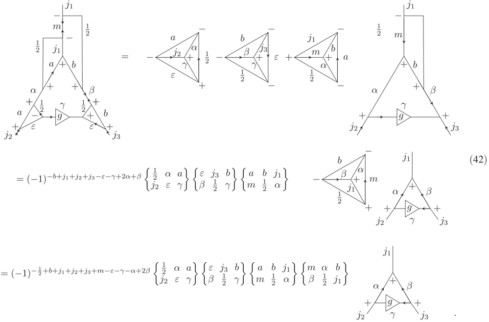
- The authors give the first complete derivation of the Euclidean Hamiltonian constraint action on 4-valent spin networks using modern graphical calculus, update the 3-valent derivation, and include the volume operator.
- Their Mathematica implementation applies the graph-changing constraint without approximations and evolves fiducial 4-valent node-like spin networks perturbatively in the lapse, up to third order when all links are allowed and up to fourth order when one link is excluded.
- Graph-preserving dynamics “miss estimates the volume expectation value both in absolute value and in the location of its minima” by nearly one order of magnitude at moderate lapse; it also violates the equality of volume profiles seen for inner virtual spins \(i=0\) and \(i=1\) under graph-changing dynamics.
- They find zero-eigenvalue eigenstates: for 3-valent spin networks, only \(j_1=j_2=j_3=0\) within the searched range; for 4-valent spin networks, the family \(j_1=j_2=j_3=j_4=i=0\). They also propose a more general family of solutions built from any desired spin network, Eq. (88).
Methods
- Analytical derivation uses SU(2) recoupling theory, Wigner \(3j\), \(6j\), and \(9j\) symbols, intertwiners, and graphical calculus to compute the action of the Euclidean scalar constraint and volume operator on 3- and 4-valent node-like spin networks.
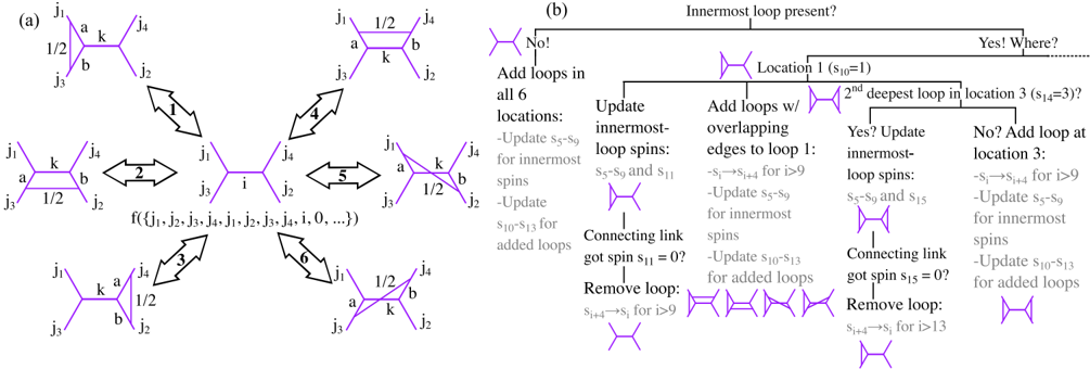
- Numerical implementation is a Mathematica code encoding spin networks as ordered lists inside “ghost functions”; the Hamiltonian constraint is a linear functional acting on these arguments, with normalizer, collector, and volume functionals.
- The unitary generated by the constraint, \(\hat U=\exp(-i\hat C_s[N])\), is expanded perturbatively in the lapse \(N\) and applied to fiducial spin networks with \(j_1=j_2=j_3=j_4=1/2\), \(\varepsilon=0\), and \(i=0\) or \(i=1\); computational times are reported, e.g. 168.8 s for \(\{1/2,1/2,1/2,1/2,0\}\) and 6543.8 s for \(\{1,1,1,1,0\}\).
Limitations
- Stated: computational-time limitations prevented completing graph-changing calculations at fourth order; the study considers only two spin networks, so the numerical data are “the first evidence” rather than a proof, and only the volume operator is used as a figure of merit.
- Stated: the work uses the Euclidean constraint, not the Lorentzian one; the physical inner product remains out of reach, the proposed solution series may not converge, and the solutions may not yet capture the full phenomenology of general relativity.
- Stated/evident: the analysis is restricted to low spins and perturbative lapse values; graph-preserving comparisons depend on the chosen spin-network structure, and the authors note that calculations at lapse values close to unity may be questionable in a perturbative study.
Model-written summary. Check it against the paper before relying on it.
Integrity signals
Registry
Cites
Statistics
Figures






Verification
Claims the paper makes
0 Valid · 3 Not valid · 27 Not checked · 178 Own results and interpretations
A result the paper reports from its own data — it cites no other source for it, so there is none to check. The quote shows it is in the paper.
In the paper
“Note that these eigenstates also include spin networks with large numbers of inner loops, as long as the innermost links meeting at the intertwiner are in the trivial representation.”
plainstates an association- Asserted: passes — The authors put it forward as true.
- Checkable: passes — It can be checked against evidence.
- Load-bearing: unclear — It is unclear whether the paper’s conclusions depend on it.
- Based: passes — The paper gives a reason why it holds.
None of the sources cited for this claim could be matched to a paper in Crossref, so there is nothing to check it against.
In the paper
“(and one of the first numerical works in canonical LQG [27 -29])”
What the sources say
- Not matchedcites [27]
Couldn’t be matched to a paper in Crossref, so it can’t be checked.
- Not matchedcites [28]
Couldn’t be matched to a paper in Crossref, so it can’t be checked.
- Not matchedcites [29]
Couldn’t be matched to a paper in Crossref, so it can’t be checked.
plain- Asserted: passes — The authors put it forward as true.
- Checkable: passes — It can be checked against evidence.
- Load-bearing: unclear — It is unclear whether the paper’s conclusions depend on it.
- Based: passes — The paper gives a reason why it holds.
- Not matched
A result the paper reports from its own data — it cites no other source for it, so there is none to check. The quote shows it is in the paper.
In the paper
“We are able to transform spin networks with graph-changing dynamics perturbatively”
plainstates a cause- Asserted: passes — The authors put it forward as true.
- Checkable: passes — It can be checked against evidence.
- Load-bearing: passes — The paper’s conclusions depend on it.
- Based: passes — The paper gives a reason why it holds.
A result the paper reports from its own data — it cites no other source for it, so there is none to check. The quote shows it is in the paper.
In the paper
“verify that the expectation values for the volume have rather different behavior from the approximated, graph-preserving results.”
- Also stated in: § II. MAIN RESULTS · p. 2 · plain
“As we anticipate in Fig. 1(c), the expectation values of the quantum volume are rather different between graph-changing and graph-preserving scenarios.”
plainstates an association- Asserted: passes — The authors put it forward as true.
- Checkable: passes — It can be checked against evidence.
- Load-bearing: passes — The paper’s conclusions depend on it.
- Based: passes — The paper gives a reason why it holds.
- Also stated in: § II. MAIN RESULTS · p. 2 · plain
A result the paper reports from its own data — it cites no other source for it, so there is none to check. The quote shows it is in the paper.
In the paper
“Furthermore, we use our code to look for low-spin eigenstates of the Euclidean Hamiltonian, showing that simple eigenstates do exist: states with only vanishing spins meeting at the intertwiner.”
boosted- Asserted: passes — The authors put it forward as true.
- Checkable: passes — It can be checked against evidence.
- Load-bearing: passes — The paper’s conclusions depend on it.
- Based: passes — The paper gives a reason why it holds.
94 more claims
Create a free account to see all 208 claims and every source verdict.
- It may state two separate claims as one. 65
- Probably not a substantial claim. 63
- The quote only partly states this claim. 1
Citations
Cites
Quantum Theory of Gravity. I. The Canonical Theory
DeWitt, B. S. (1967) · Physical Review · doi:10.1103/physrev.160.1113 · Cited by 3,385
Breakdown of predictability in gravitational collapse
Hawking, S. W. (1976) · Physical Review D · doi:10.1103/physrevd.14.2460 · Cited by 2,554
Rovelli, C. (2004) · doi:10.1017/cbo9780511755804 · Cited by 2,240
Modern Canonical Quantum General Relativity
Thiemann, T. (2007) · doi:10.1017/cbo9780511755682 · Cited by 2,001
Background independent quantum gravity: a status report
Ashtekar, A., & Lewandowski, J. (2004) · Classical and Quantum Gravity · doi:10.1088/0264-9381/21/15/r01 · Cited by 1,951
New Variables for Classical and Quantum Gravity
Ashtekar, A. (1986) · Physical Review Letters · doi:10.1103/physrevlett.57.2244 · Cited by 1,663
Loop quantum cosmology: a status report
Ashtekar, A., & Singh, P. (2011) · Classical and Quantum Gravity · doi:10.1088/0264-9381/28/21/213001 · Cited by 1,205
State sum invariants of 3-manifolds and quantum 6j-symbols
Turaev, V. G., & Viro, O. Y. (1992) · Topology · doi:10.1016/0040-9383(92)90015-a · Cited by 1,145
Quantum theory of geometry: I. Area operators
Ashtekar, A., & Lewandowski, J. (1997) · Classical and Quantum Gravity · doi:10.1088/0264-9381/14/1a/006 · Cited by 852
Loop space representation of quantum general relativity
Rovelli, C., & Smolin, L. (1990) · Nuclear Physics B · doi:10.1016/0550-3213(90)90019-a · Cited by 806
Research works printed but not linked: 3
- P. A. M. Dirac, 2001, Lectures on Quantum Mechanics
- D. Brink, 1968, Angular Momentum
- A. Messiah, 1962, Quantum Mechanics Vol. II
Cited by
Computing the Graph-Changing Dynamics of Loop Quantum Gravity
Guedes, T. L. M., Marugán, G. A. M., Vidotto, F., & Müller, M. (2025) · Universe · doi:10.3390/universe11120387 · Cited by 9
“In this context, the different volume profiles in GC and GP approaches can have great influence in cosmology [42, 46], leading to different expansion rates and inflationary regimes, or in black hole evolution, modifying the black-to-white hole transition time [47, 48].”
InfluentialSelf-citationConsciousness Emergent from Information Networks
Bi, Q. (2026) · Journal of Quantum Information Science · doi:10.4236/jqis.2026.162011
Elementary blocks of loop quantum gravity
Assanioussi, M., & Livine, E. R. (2026) · Classical and Quantum Gravity · doi:10.1088/1361-6382/ae910e · Cited by 4
Sahlmann, H., & Sherif, W. (2026) · Classical and Quantum Gravity · doi:10.1088/1361-6382/aea5cb · Cited by 2
“Recently, among attempts to approach this problem [20–24], a complementary direction has started to look practicable whereby one treats a truncated, fixed-graph kinematical Hilbert space as a large, but finite, many-body system [30].”
Time evolution of semiclassical states in the one-vertex model of quantum-reduced loop gravity
Mäkinen, I. H. (2026) · The European Physical Journal C · doi:10.1140/epjc/s10052-026-15969-6 · Cited by 3
Metadata
- Authors
- Guedes, T. L. M., Mena Marugán, G. A., Müller, M., & Vidotto, F.
- Affiliations
- Forschungszentrum Jülich (DE)
- Instituto de Estructura de la Materia, IEM-CSIC
- Western University (CA)
- Venue
- Physical Review D
- Publisher
- American Physical Society (APS)
- Published
- 2025-07-22
- Volume
- 112
- Issue
- 2
- ISSN
- 2470-0010 (ISSN-L)
- 2470-0029
- OpenAlex
- W4411630364
- Semantic Scholar
- 7f414721afb4703e50972a12ea9db8f2fea7e735
- Cited by
- 5
- References
- 61
- Citations by year
- 2026: 4 · 2025: 1
- FWCI
- 2.06
- Type
- journal article
- Language
- en
- Open access
- hybrid
- doi.org
- Licence
- Locations
- Physical review. D/Physical review. D. (publishedVersion, cc-by)
- DIGITAL.CSIC (Spanish National Research Council (CSIC)) (submittedVersion, cc-by)
- Funders
- John Templeton Foundation (62312)
- European Research Council (804247)
- HORIZON EUROPE European Research Council (101114305, 101046968)
- Deutsche Forschungsgemeinschaft
- Canada Excellence Research Chairs, Government of Canada
- Natural Sciences and Engineering Research Council of Canada
- Institut Périmètre de physique théorique
- Government of Canada
- Industry Canada
- Ontario Ministry of Economic Development and Innovation
- Ministerio de Ciencia e Innovación
- Agencia Estatal de Investigación
- Federación Española de Enfermedades Raras (PID2020-118159GB-C41)
- Ministerio de Ciencia, Innovación y Universidades (PID2023-149018NB-C41)
- European Social Fund Plus
- Cluster of Excellence Matter and Light for Quantum Computing (EXC 2004/1, 390534769)
- Hightech Agenda Bayern Plus
- Topics
- Physical Sciences › Physics and Astronomy › Nuclear and High Energy Physics › Noncommutative and Quantum Gravity Theories
- Physical Sciences › Physics and Astronomy › Astronomy and Astrophysics › Relativity and Gravitational Theory
- Physical Sciences › Physics and Astronomy › Nuclear and High Energy Physics › Black Holes and Theoretical Physics
- Keywords
- loop quantum gravity, Hamiltonian constraint, spin networks, physical Hilbert space, eigenstates, volume operator, expectation values, reversibility, physical subspace
About these checks
Registry, retraction, Cites and statistics results are computed, not judged, with one exception: a printed reference that no index lists is read once by a model before it counts as a citation error. Claims are extracted by a model and kept only when their quote appears verbatim in the text; each cited source is then checked, with a model’s help, for whether it says what the claim relies on. Those verdicts can be wrong — read the claim’s quote and the cited source before relying on one.
A language model drew the claims from the paper on 2026-10-29, under version 3 of the claim definition (model deepseek-v4.1-flash, prompt extract-v3).
A second model labelled each claim on 2026-10-29 (model jev-1.13-20260917, definition revision gold-guideline-v0.2).
Statistics and arithmetic are recomputed, not judged.
Confidence bands are shown only for fields calibrated on our annotated test set. None is calibrated yet, so no band is shown.
What counts as a claim ›How we measure confidence ›How we check this ›
Are you an author, or do you see a problem with this page? Request a review
How to cite
Cite CoChat for the checks on this page, and the paper for its own findings.
- This page
- CoChat. (2026). Citation check: Taming Thiemann’s Hamiltonian constraint in canonical loop quantum gravity: Reversibility, eigenstates, and graph-change analysis. https://app.cochat.ai/papers/10.1103/hjdk-kdhk
- The paper
- Guedes, T. L. M., Mena Marugán, G. A., Müller, M., & Vidotto, F. (2025). Taming Thiemann’s Hamiltonian constraint in canonical loop quantum gravity: Reversibility, eigenstates, and graph-change analysis. Physical Review D. https://doi.org/10.1103/hjdk-kdhk
Data sources
Bibliographic data: Semantic Scholar, OpenAlex, Crossref.
Contains information from the Semantic Scholar Academic Graph Datasets, made available under the ODC Attribution License (ODC-BY 1.0).
Semantic Scholar’s data is described in: Kinney, R., et al. (2023). The Semantic Scholar Open Data Platform. arXiv:2301.10140.
