Cited by 257Computational Drug Discovery MethodsTopological and Geometric Data AnalysisMachine Learning in Bioinformatics

The DOI matches its Crossref record; 143 of the 143 references it cites were found in a registry or an index.

Representability of algebraic topology for biomolecules in machine learning based scoring and virtual screening

Open access
Cang, Zixuan, Mu, Lin, Wei, Guo-Wei·2018·PLOS Computational Biology

Abstract

This work introduces a number of algebraic topology approaches, including multi-component persistent homology, multi-level persistent homology, and electrostatic persistence for the representation, characterization, and description of small molecules and biomolecular complexes. In contrast to the conventional persistent homology, multi-component persistent homology retains critical chemical and biological information during the topological simplification of biomolecular geometric complexity. Multi-level persistent homology enables a tailored topological description of inter- and/or intra-molecular interactions of interest. Electrostatic persistence incorporates partial charge information into topological invariants. These topological methods are paired with Wasserstein distance to characterize similarities between molecules and are further integrated with a variety of machine learning algorithms, including k-nearest neighbors, ensemble of trees, and deep convolutional neural networks, to manifest their descriptive and predictive powers for protein-ligand binding analysis and virtual screening of small molecules. Extensive numerical experiments involving 4,414 protein-ligand complexes from the PDBBind database and 128,374 ligand-target and decoy-target pairs in the DUD database are performed to test respectively the scoring power and the discriminatory power of the proposed topological learning strategies. It is demonstrated that the present topological learning outperforms other existing methods in protein-ligand binding affinity prediction and ligand-decoy discrimination.

Overview

The claims and statistics of this paper haven’t been checked yet.

Run the check — free, no account needed. It reads the open-access text and checks the sources it cites.

A few free checks a day · papers already verified open instantly · results are public

Integrity signals

Registry

Crossref · 10.1371/journal.pcbi.1005929

Cites

143 of 143 references verified0 citation errors · 0 not checkable

Statistics

Figures

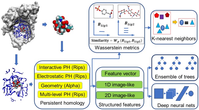
Fig 1 An illustration of the topology based machine learning algorithms used in scoring and virtual screening.
Fig 1 An illustration of the topology based machine learning algorithms used in scoring and virtual screening.CC BY · PubMed Central
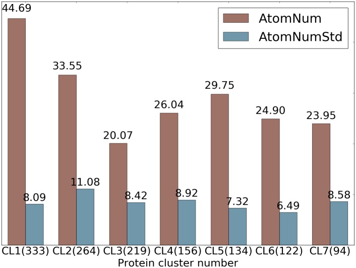
Fig 2 Statistics of ligands in 7 protein clusters in S1322 dataset. The average numbers of heavy atoms of a ligand in each protein cluster are shown in red and the standard deviations of number of heavy atoms across each protein cluster are shown in blue. The number of ligands in each cluster is given in parentheses.
Fig 2 Statistics of ligands in 7 protein clusters in S1322 dataset. The average numbers of heavy atoms of a ligand in each protein cluster are shown in red and the standard deviations of number of heavy atoms across each protein cluster are shown in blue. The number of ligands in each cluster is given in parentheses.CC BY · PubMed Central
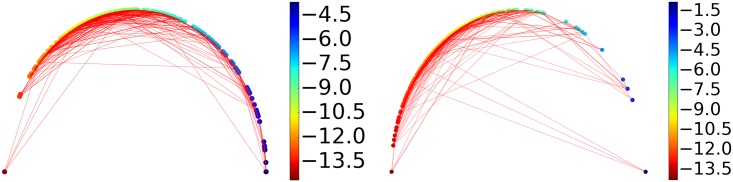
Fig 3 An illustration of similarities between ligands measured by their barcode space Wasserstein distances. Ligands are ordered according to their binding affinities and are represented as dots on the semicircle. Specifically, a sample of binding free energy x is plotted at the angle θ = π(Emax − x)/(Emax − Emin) where Emin and Emax are the lowest and the highest energy in the dataset. Each dot is connected with two nearest neighbors based on their barcode space Wasserstein distances. An optimal prediction would be achieved if lines stay close to the semicircle. The majority of the connections stay near the boundary to the upper half sphere demonstrating that barcode space metric based Wasserstein distance measurement reflects the similarity in function, i.e., the binding affinity in this case. The protein clusters with the best and the worst performance are shown. Left: Protein cluster 2. Right: Protein cluster 3.
Fig 3 An illustration of similarities between ligands measured by their barcode space Wasserstein distances. Ligands are ordered according to their binding affinities and are represented as dots on the semicircle. Specifically, a sample of binding free energy x is plotted at the angle θ = π(Emax − x)/(Emax − Emin) where Emin and Emax are the lowest and the highest energy in the dataset. Each dot is connected with two nearest neighbors based on their barcode space Wasserstein distances. An optimal prediction would be achieved if lines stay close to the semicircle. The majority of the connections stay near the boundary to the upper half sphere demonstrating that barcode space metric based Wasserstein distance measurement reflects the similarity in function, i.e., the binding affinity in this case. The protein clusters with the best and the worst performance are shown. Left: Protein cluster 2. Right: Protein cluster 3.CC BY · PubMed Central
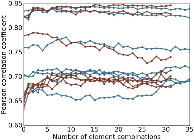
Fig 4 Plot of performance against number of element combinations used. The topological learning model performance against the number of element combinations involved in feature construction for 7 protein clusters in S1322. The horizontal axis corresponds to the number of element combinations used for the features. From left to right, one extra element combination is added at a step. The features are then used in gradient boosting trees method to test if the model is robust against redundant information. The results related to alpha complex are marked in red and Rips complex in blue. The median Pearson correlation coefficient between predicted and experimental results is reported of 10-fold cross-validation within each protein cluster repeated 20 times are reported.
Fig 4 Plot of performance against number of element combinations used. The topological learning model performance against the number of element combinations involved in feature construction for 7 protein clusters in S1322. The horizontal axis corresponds to the number of element combinations used for the features. From left to right, one extra element combination is added at a step. The features are then used in gradient boosting trees method to test if the model is robust against redundant information. The results related to alpha complex are marked in red and Rips complex in blue. The median Pearson correlation coefficient between predicted and experimental results is reported of 10-fold cross-validation within each protein cluster repeated 20 times are reported.CC BY · PubMed Central
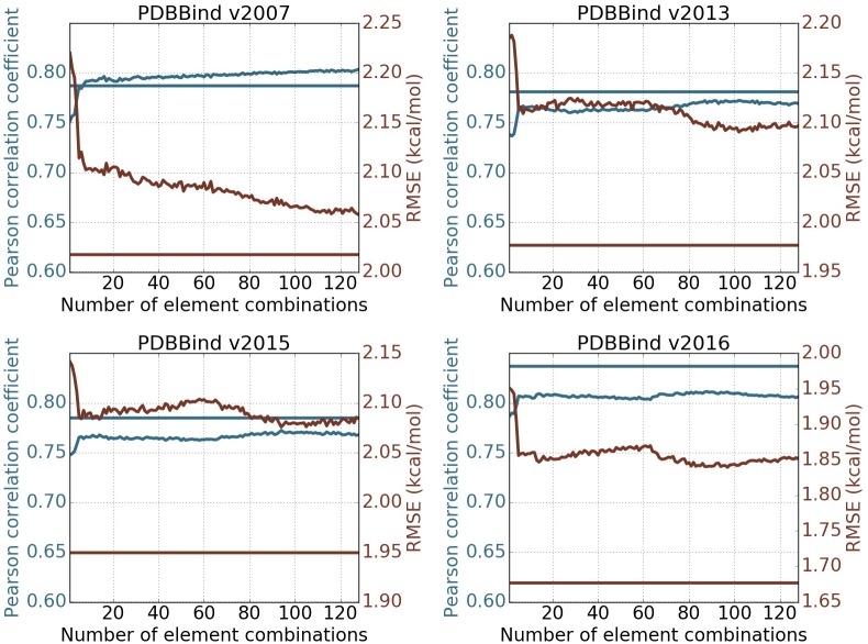
Fig 5 Feature robustness tests on PDBBind datasets. The performance of the topological learning model against the number of included element combinations for predicting on PDBBind core sets and training on PDBBind refined sets minus the core sets. The 1st and 2nd dimensional barcodes computed with alpha complex is used. Features are generated following barcode statistics method. Element combinations are all possible paired choices of one item from {C, N, O, CN, CO, NO, CNO, CNOS} in protein and another item from {C, N, O, S, CN, CO, CS, NO, NS, OS, CNO, CNS, COS, NOS, CNOS, CNOSPFClBrI} in ligand, which result in 128 element combinations. The horizontal straight lines represents the performance of the 2D representation with deep convolutional neural network (row 10 in Table 10). The blue and red colors correspond to Pearson correlation coefficient and RMSE (kcal/mol) respectively. Each experiment is done by training on refined set minus the core set with the median result of 20 repeated runs reported.
Fig 5 Feature robustness tests on PDBBind datasets. The performance of the topological learning model against the number of included element combinations for predicting on PDBBind core sets and training on PDBBind refined sets minus the core sets. The 1st and 2nd dimensional barcodes computed with alpha complex is used. Features are generated following barcode statistics method. Element combinations are all possible paired choices of one item from {C, N, O, CN, CO, NO, CNO, CNOS} in protein and another item from {C, N, O, S, CN, CO, CS, NO, NS, OS, CNO, CNS, COS, NOS, CNOS, CNOSPFClBrI} in ligand, which result in 128 element combinations. The horizontal straight lines represents the performance of the 2D representation with deep convolutional neural network (row 10 in Table 10). The blue and red colors correspond to Pearson correlation coefficient and RMSE (kcal/mol) respectively. Each experiment is done by training on refined set minus the core set with the median result of 20 repeated runs reported.CC BY · PubMed Central
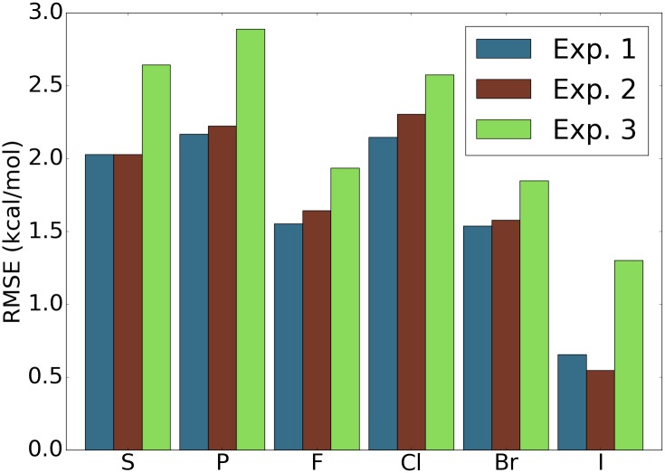
Fig 6 Assessment of performance of the model on samples with elements that are rare in the data sets. For the four data sets PDBBind v2007, v2013, v2015, and v2016 [99], and for each element, the testing set is the subset of the original core sets with only ligands that contain atoms of the particular element type. The features used are features with ID = 7 in Table 10. The reported RMSE is the average taken over the four data sets. Experiment 1: Training set is the original training set and all the features are used. Experiment 2: Training set is the original training set and only features that do not involve the particular element are used. Experiment 3: Training set is the original training set excluding the samples that contain atoms of the particular element type and all features are used. For most of the elements, experiment 1 achieves the best result and experiment 3 yields the worst performance.
Fig 6 Assessment of performance of the model on samples with elements that are rare in the data sets. For the four data sets PDBBind v2007, v2013, v2015, and v2016 [99], and for each element, the testing set is the subset of the original core sets with only ligands that contain atoms of the particular element type. The features used are features with ID = 7 in Table 10. The reported RMSE is the average taken over the four data sets. Experiment 1: Training set is the original training set and all the features are used. Experiment 2: Training set is the original training set and only features that do not involve the particular element are used. Experiment 3: Training set is the original training set excluding the samples that contain atoms of the particular element type and all features are used. For most of the elements, experiment 1 achieves the best result and experiment 3 yields the worst performance.CC BY · PubMed Central
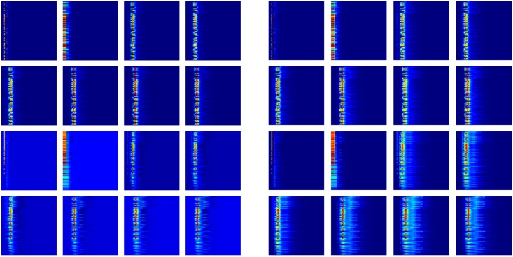
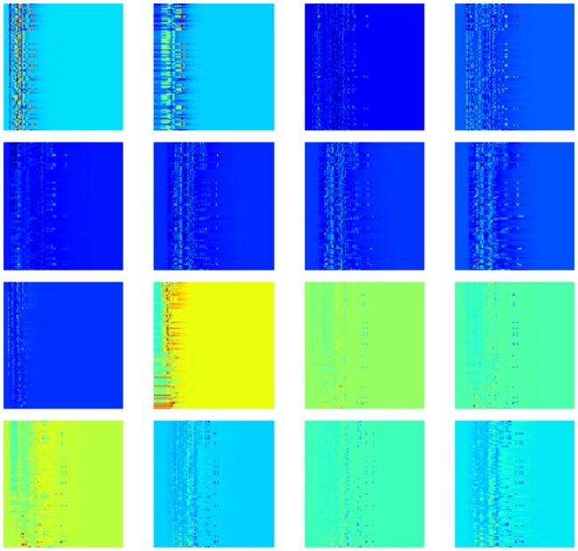
Fig 7 Heat map plot of the 16 channels. The mean value (left image) and the standard deviation (right image) of each digit over the PDBBind v2016 refined set are shown. The top 8 maps are for protein-ligand complex and the other 8 maps are for the difference between protein-ligand complex and protein only. For each map, the vertical axis is the element combinations ordered according to their importance and the horizontal axis is the dimension of spatial scales.
Fig 7 Heat map plot of the 16 channels. The mean value (left image) and the standard deviation (right image) of each digit over the PDBBind v2016 refined set are shown. The top 8 maps are for protein-ligand complex and the other 8 maps are for the difference between protein-ligand complex and protein only. For each map, the vertical axis is the element combinations ordered according to their importance and the horizontal axis is the dimension of spatial scales.CC BY · PubMed Central
Fig 8 Multi-level persistent homology on simple small molecules. Illustration of representation ability of M˜ in reflecting structural perturbations among conformations of the same molecule. Left: The structural alignment of two conformations of the ligand in protein-ligand complex (PDB:1BCD). Right: The persistence diagram showing the 1st and 2nd dimensional results generated using Rips complex with M˜ for two conformations. It is worth noticing that the barcodes generated using Rips complex with M are identical for the two conformations.
Fig 8 Multi-level persistent homology on simple small molecules. Illustration of representation ability of M˜ in reflecting structural perturbations among conformations of the same molecule. Left: The structural alignment of two conformations of the ligand in protein-ligand complex (PDB:1BCD). Right: The persistence diagram showing the 1st and 2nd dimensional results generated using Rips complex with M˜ for two conformations. It is worth noticing that the barcodes generated using Rips complex with M are identical for the two conformations.CC BY · PubMed Central
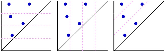
Fig 9 Illustration of dividing set of barcodes into subsets. The barcodes are plotted as persistence diagrams with the horizontal axis being birth and the vertical axis being death. From left to right, the subsets are generated according to the slicing of death, birth, and persistence values.
Fig 9 Illustration of dividing set of barcodes into subsets. The barcodes are plotted as persistence diagrams with the horizontal axis being birth and the vertical axis being death. From left to right, the subsets are generated according to the slicing of death, birth, and persistence values.CC BY · PubMed Central
Fig 10 The 2D topological maps of the 16 channels of sample 1wkm. The top 8 maps are for protein-ligand complex and the other 8 maps are for the difference between protein-ligand complex and protein only. For each map, the horizontal axis is the dimension of spatial scale and the vertical axis is element combinations ordered by their importance.
Fig 10 The 2D topological maps of the 16 channels of sample 1wkm. The top 8 maps are for protein-ligand complex and the other 8 maps are for the difference between protein-ligand complex and protein only. For each map, the horizontal axis is the dimension of spatial scale and the vertical axis is element combinations ordered by their importance.CC BY · PubMed Central
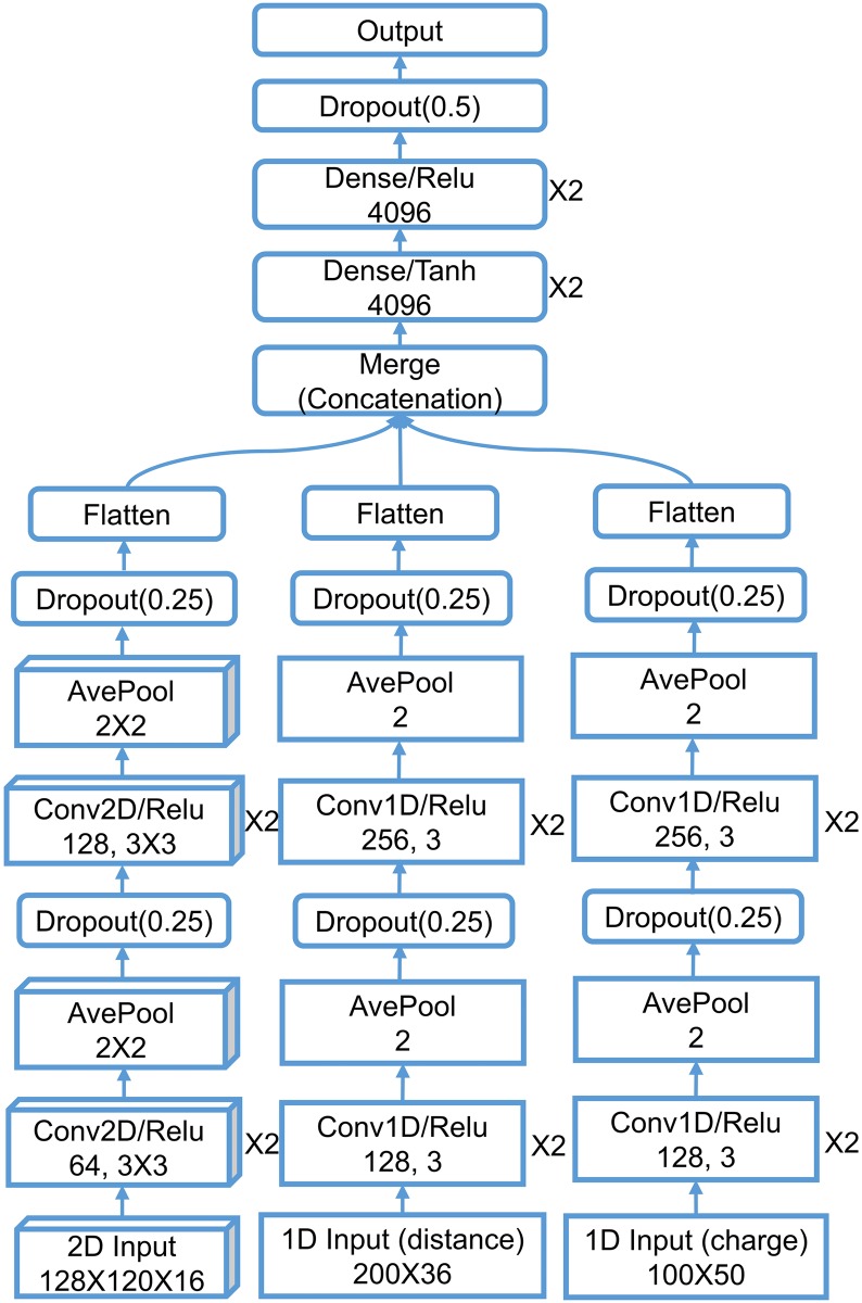
Fig 11 The network architecture of TopBP-DL. The structured layers are shown in boxes/rectangles with sharp corners for 2D/1D image-like content and the unstructured layers are shown in rectangles. The numbers in convolution layers mean the number of filters and filter size from left to right. The dense layers are drawn with number of neurons and activation function. The pooling size of the pooling layers and dropout rate of the dropout layers are listed. The layers that are repeated n times are marked with “×n” sign on the right side of the layer.
Fig 11 The network architecture of TopBP-DL. The structured layers are shown in boxes/rectangles with sharp corners for 2D/1D image-like content and the unstructured layers are shown in rectangles. The numbers in convolution layers mean the number of filters and filter size from left to right. The dense layers are drawn with number of neurons and activation function. The pooling size of the pooling layers and dropout rate of the dropout layers are listed. The layers that are repeated n times are marked with “×n” sign on the right side of the layer.CC BY · PubMed Central
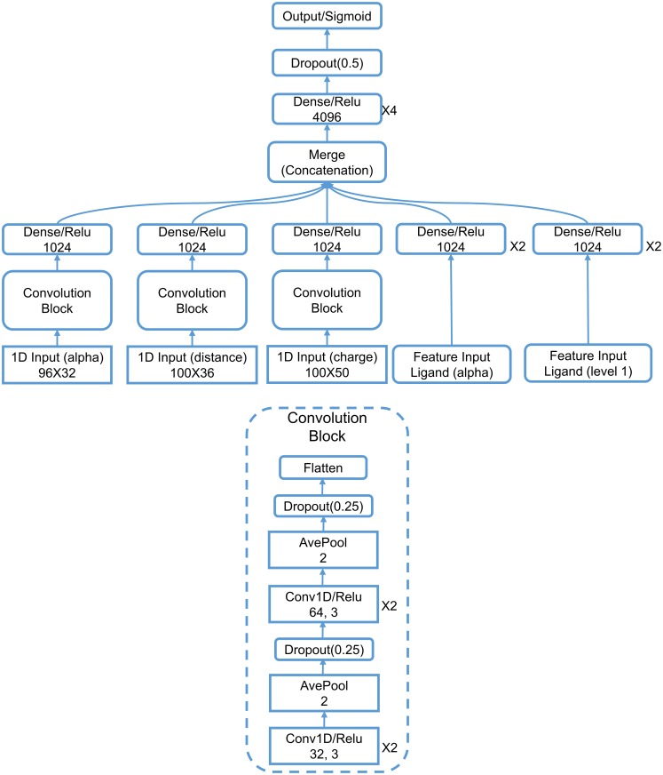
Fig 12 The network architecture of TopVS-DL. The 1D image-like layers are shown in sharp-corner rectangles. The numbers in convolution layers mean the number of filters and filter size from left to right. The pooling size of the pooling layers and dropout rate of the dropout layers are listed. The layers that are repeated n times are marked with “×n” sign on the right side of the layer.
Fig 12 The network architecture of TopVS-DL. The 1D image-like layers are shown in sharp-corner rectangles. The numbers in convolution layers mean the number of filters and filter size from left to right. The pooling size of the pooling layers and dropout rate of the dropout layers are listed. The layers that are repeated n times are marked with “×n” sign on the right side of the layer.CC BY · PubMed Central

Verification

Claims the paper makes

The claims and statistics of this paper haven’t been checked yet.

Run the check — free, no account needed. It reads the open-access text and checks the sources it cites.

A few free checks a day · papers already verified open instantly · results are public

Claims other papers make about this one

Each is checked against this paper’s own text: does it say what the citing paper says it does?

Self-check

Percentages, sums and reported differences re-computed from the paper’s own numbers.

The self-check needs the paper’s full text.

Citations

Cites

Show all 140 references

Research works printed but not linked: 6

  1. Q Zheng, 2012, Molecular surface generation using PDE transform, International Journal for Numerical Methods in Biomedical Engineering, 28, 291
  2. X Shi, 2011, Geometry and topology for modeling biomolecular surfaces, Far East J Applied Math, 50, 1
  3. T Kaczynski, 2004, vol. 157 of Applied Mathematical Sciences
  4. VD Silva, 2005, In Proceedings of Robotics: Science and Systems, 01
  5. B Krishnamoorthy, 2007, Data Mining in Biomedicine, Springer Optimization and Its Applications, 431
  6. PM Kasson, 2007, Persistent voids: a new structural metric for membrane fusion, Bioinformatics, 23, 1753, 10.1093/bioinformatics/btm250 · DOI

Cited by

Sorted by citations

See all 257

Metadata

Authors
Cang, Z., Mu, L., & Wei, G.-W.
Affiliations
  • Michigan State University (US)
  • Oak Ridge National Laboratory (US)
Corresponding author
Wei, Guo-Wei
Venue
PLOS Computational Biology
Published
2018-01-08
Volume
14
Issue
1
Pages
e1005929
ISSN
  • 1553-734X (ISSN-L)
  • 1553-7358
OpenAlex
W2963833291
Cited by
257
References
140
Citations by year
2026: 21 · 2025: 34 · 2024: 28 · 2023: 37 · 2022: 35 · 2021: 35 · 2020: 39 · 2019: 17 · 2018: 11
FWCI
18.85
Type
journal article
Language
en
Open access
Locations
  • PLoS Computational Biology (publishedVersion, cc-by)
  • Europe PMC (PubMed Central) (publishedVersion, cc-by)
  • PubMed Central (publishedVersion, cc-by)
  • PubMed (publishedVersion)
  • arXiv (Cornell University) (submittedVersion)
  • OSTI OAI (U.S. Department of Energy Office of Scientific and Technical Information) (submittedVersion)
  • RePEc: Research Papers in Economics (submittedVersion)
  • DOAJ (DOAJ: Directory of Open Access Journals) (submittedVersion, cc-by-sa)
  • arXiv (Cornell University)
Funders
National Science Foundation (DMS-1721024, IIS-1302285)
Topics
  • Life Sciences › Pharmacology, Toxicology and Pharmaceutics › Drug Discovery › Computational Drug Discovery Methods
  • Physical Sciences › Computer Science › Computational Theory and Mathematics › Topological and Geometric Data Analysis
  • Life Sciences › Biochemistry, Genetics and Molecular Biology › Molecular Biology › Machine Learning in Bioinformatics
Keywords
algebraic topology, persistent homology, Wasserstein distance, protein-ligand binding affinity prediction, virtual screening, biomolecular complexes, PDBbind
MeSH terms
Machine Learning, Algorithms, Humans, Ligands, Models, Neurological, Nucleic Acids, Protein Binding, Proteins, Neural Networks, Computer, Computational Biology, Area Under Curve, Protein Interaction Mapping, Databases, Protein, Static Electricity, Molecular Dynamics Simulation

About these checks

Registry, retraction, Cites and statistics results are computed, not judged, with one exception: a printed reference that no index lists is read once by a model before it counts as a citation error. Claims are extracted by a model and kept only when their quote appears verbatim in the text; each cited source is then checked, with a model’s help, for whether it says what the claim relies on. Those verdicts can be wrong — read the claim’s quote and the cited source before relying on one.

Statistics and arithmetic are recomputed, not judged.

Confidence bands are shown only for fields calibrated on our annotated test set. None is calibrated yet, so no band is shown.

What counts as a claim ›How we measure confidence ›How we check this ›

Are you an author, or do you see a problem with this page? Request a review