PreprintCited by 10Advanced Physical and Chemical Molecular InteractionsProtein Structure and DynamicsAdvanced Chemical Physics Studies

The DOI matches its Crossref record; 1 of the 1 references it cites were found in a registry or an index.

"Dividing and Conquering" and "Caching" in Molecular Modeling

Open access
Cao, Xiaoyong, Tian, Pu·2021·International Journal of Molecular Sciences

Preprint — published as 10.3390/ijms22095053 · Paper page

Abstract

Molecular modeling is widely utilized in subjects including but not limited to physics, chemistry, biology, materials science and engineering. Impressive progress has been made in development of theories, algorithms and software packages. To divide and conquer, and to cache intermediate results have been long standing principles in development of algorithms. Not surprisingly, Most of important methodological advancements in more than half century of molecule modeling are various implementations of these two fundamental principles. In the mainstream classical computational molecular science based on force fields parameterization by coarse graining, tremendous efforts have been invested on two lines of algorithm development. The first is coarse graining, which is to represent multiple basic particles in higher resolution modeling as a single larger and softer particle in lower resolution counterpart, with resulting force fields of partial transferability at the expense of some information loss. The second is enhanced sampling, which realizes "dividing and conquering" and/or "caching" in configurational space with focus either on reaction coordinates and collective variables as in metadynamics and related algorithms, or on the transition matrix and state discretization as in Markov state models. For this line of algorithms, spatial resolution is maintained but no transferability is available. Deep learning has been utilized to realize more efficient and accurate ways of "dividing and conquering" and "caching" along these two lines of algorithmic research. We proposed and demonstrated the local free energy landscape approach, a new framework for classical computational molecular science and a third class of algorithm that facilitates molecular modeling through partially transferable in resolution "caching" of distributions for local clusters of molecular degrees of freedom. Differences, connections and potential interactions among these three algorithmic directions are discussed, with the hope to stimulate development of more elegant, efficient and reliable formulations and algorithms for "dividing and conquering" and "caching" in complex molecular systems.

Overview

The claims and statistics of this paper haven’t been checked yet.

Run the check — free, no account needed. It reads the open-access text and checks the sources it cites.

A few free checks a day · papers already verified open instantly · results are public

Integrity signals

Registry

Crossref · 10.20944/preprints202012.0081.v2

Cites

1 of 1 references verified0 citation errors · 0 not checkable

Statistics

Figures

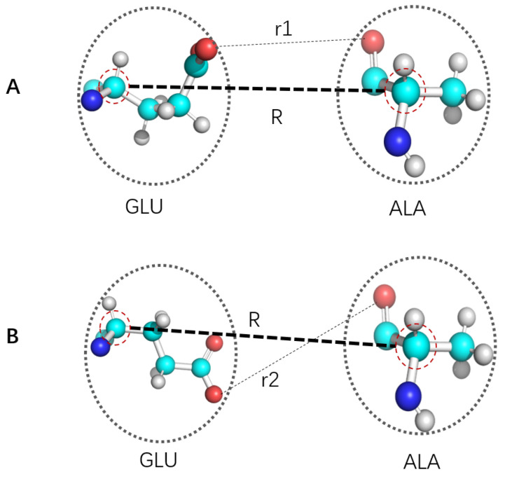
Figure 1 Schematic illustration of time scale separation issue in CG. (A,B) show two situations with Cα distances between two amino acids GLU and ALA being R, but with GLU have different conformations. If Cα atoms were defined as CG site, then these two relative conformation with distinct interactions would be treated as the same. In (A,B), CG site distance in both (A,B) are R, but many other pairs of atoms have distinct distances as exemplified by r1 and r2. Such treatment would only be true if for any small amount of displacement of Cα, side chains accomplished many rotations and thus may be accurately represented by averaging (i.e., with good time scale separation). This issue is apparently not limited to the specific definition of Cα being CG site, but rather general for essentially all CG development.
Figure 1 Schematic illustration of time scale separation issue in CG. (A,B) show two situations with Cα distances between two amino acids GLU and ALA being R, but with GLU have different conformations. If Cα atoms were defined as CG site, then these two relative conformation with distinct interactions would be treated as the same. In (A,B), CG site distance in both (A,B) are R, but many other pairs of atoms have distinct distances as exemplified by r1 and r2. Such treatment would only be true if for any small amount of displacement of Cα, side chains accomplished many rotations and thus may be accurately represented by averaging (i.e., with good time scale separation). This issue is apparently not limited to the specific definition of Cα being CG site, but rather general for essentially all CG development.CC BY · PubMed Central
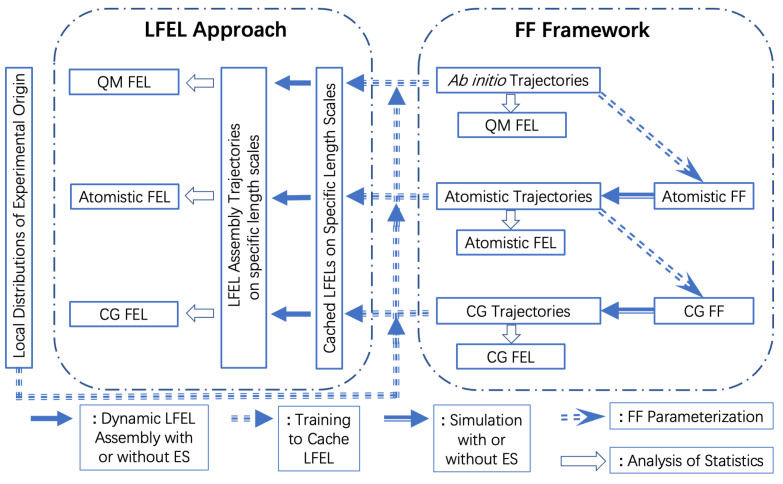
Figure 2 Schematic illustration of the LFEL approach in contrast to present mainstream FF framework. FF parameterization is the foundation for present classical computational molecular science. Training of neural network for “caching” LFEL is the foundation for LFEL approach, the source data can be either of experimental or computational origin. In FF framework, simulation (with or without ES) is driven by FF, in LFEL approach, propagation of molecular systems to minimize free energy (or maximize joint probability) is driven by compromise among many LFELs. Expensive repetitive local sampling in FF framework is substituted by differentiation w.r.t. LFELs.
Figure 2 Schematic illustration of the LFEL approach in contrast to present mainstream FF framework. FF parameterization is the foundation for present classical computational molecular science. Training of neural network for “caching” LFEL is the foundation for LFEL approach, the source data can be either of experimental or computational origin. In FF framework, simulation (with or without ES) is driven by FF, in LFEL approach, propagation of molecular systems to minimize free energy (or maximize joint probability) is driven by compromise among many LFELs. Expensive repetitive local sampling in FF framework is substituted by differentiation w.r.t. LFELs.CC BY · PubMed Central
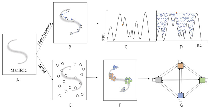
Figure 3 Schematic illustration of essential features for enhanced sampling by metadynamics and MSM. (A) The “S” shape grey line represents the unknown manifold in the configurational space (represented by the square) of a molecular system. (B) Small circles connected by blue arrows represent computed (guessed) RC/CVs for the molecular system, which is utilized to conduct metadynamics simulations. (C) The FEL of the molecular system along the computed/selected RC/CV in (B,D) “Caching” of the LFEL by bias potentials (gaussians represented by blue bell shaped lines) accumulated in the course of metadynamics simulations. (E) Distribution of the molecular system to the whole configurational space at the start of a MSM simulation, small circles represent initial start points for short MSM trajectories. (F) Sampling results of short MSM trajectories fall mainly near the manifold, distinct “states” are represented by different colors. (G) Establishment of transition matrix by transition counts between “states” obtained from short trajectories.
Figure 3 Schematic illustration of essential features for enhanced sampling by metadynamics and MSM. (A) The “S” shape grey line represents the unknown manifold in the configurational space (represented by the square) of a molecular system. (B) Small circles connected by blue arrows represent computed (guessed) RC/CVs for the molecular system, which is utilized to conduct metadynamics simulations. (C) The FEL of the molecular system along the computed/selected RC/CV in (B,D) “Caching” of the LFEL by bias potentials (gaussians represented by blue bell shaped lines) accumulated in the course of metadynamics simulations. (E) Distribution of the molecular system to the whole configurational space at the start of a MSM simulation, small circles represent initial start points for short MSM trajectories. (F) Sampling results of short MSM trajectories fall mainly near the manifold, distinct “states” are represented by different colors. (G) Establishment of transition matrix by transition counts between “states” obtained from short trajectories.CC BY · PubMed Central
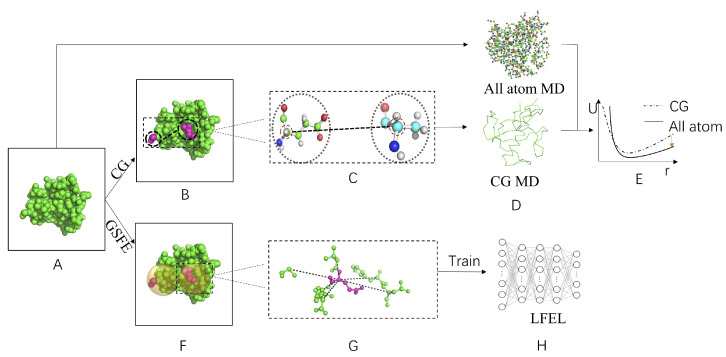
Figure 4 Schematic illustration of difference between CG and GSFE implementation of LFEL using protein as an example. (A) Target molecular systems in physical space. Due to the goal of constructing partially transferable models and/or force fields, usually many different but similar molecular systems are considered. (B) Selection of local atom/particle clusters to be represented as one particle in CG model. (C) Selection of CG sites. (D) Comparison between atomistic (or higher resolution) simulation results and CG (lower resolution) results. (E) Adjust of CG FF parameter according to comparison from (D). (F) Definition of solvent region for each solute unit. (G) Feature extraction for each solute. (H) “Caching” of LFEL with neural network by training with prepared data sets.
Figure 4 Schematic illustration of difference between CG and GSFE implementation of LFEL using protein as an example. (A) Target molecular systems in physical space. Due to the goal of constructing partially transferable models and/or force fields, usually many different but similar molecular systems are considered. (B) Selection of local atom/particle clusters to be represented as one particle in CG model. (C) Selection of CG sites. (D) Comparison between atomistic (or higher resolution) simulation results and CG (lower resolution) results. (E) Adjust of CG FF parameter according to comparison from (D). (F) Definition of solvent region for each solute unit. (G) Feature extraction for each solute. (H) “Caching” of LFEL with neural network by training with prepared data sets.CC BY · PubMed Central

Verification

Claims the paper makes

The claims and statistics of this paper haven’t been checked yet.

Run the check — free, no account needed. It reads the open-access text and checks the sources it cites.

A few free checks a day · papers already verified open instantly · results are public

Self-check

Percentages, sums and reported differences re-computed from the paper’s own numbers.

The self-check needs the paper’s full text.

Citations

Cites

Metadata

Authors
Cao, X., & Tian, P.
Affiliations
Jilin University (CN)
Corresponding author
Tian, Pu
Venue
International Journal of Molecular Sciences
Publisher
MDPI AG
Published
2021-01-05
Volume
22
Issue
9
Pages
5053-5053
ISSN
1422-0067 (ISSN-L)
OpenAlex
W3162742939
Cited by
10
References
1
Citations by year
2024: 2 · 2023: 1 · 2022: 1 · 2021: 6
FWCI
0.26
Type
journal article
Language
en
Open access
Locations
  • International Journal of Molecular Sciences (publishedVersion, cc-by)
  • Preprints.org (acceptedVersion, cc-by)
  • PubMed Central (publishedVersion, cc-by)
  • PubMed (publishedVersion)
  • DOAJ (DOAJ: Directory of Open Access Journals) (submittedVersion, cc-by-sa)
Funders
  • National Natural Science Foundation of China (2017YFB0702500, 31270758)
  • National Key Research and Development Program of China (2017YFB0702500)
Topics
  • Physical Sciences › Chemistry › Physical and Theoretical Chemistry › Advanced Physical and Chemical Molecular Interactions
  • Life Sciences › Biochemistry, Genetics and Molecular Biology › Molecular Biology › Protein Structure and Dynamics
  • Physical Sciences › Physics and Astronomy › Atomic and Molecular Physics, and Optics › Advanced Chemical Physics Studies
Keywords
coarse-graining, enhanced sampling, metadynamics, Markov state models, deep learning, free energy distribution, configurational sampling, reaction coordinate, collective variables, transferability
MeSH terms
Algorithms, Models, Molecular, Thermodynamics, Molecular Dynamics Simulation

About these checks

Registry, retraction, Cites and statistics results are computed, not judged, with one exception: a printed reference that no index lists is read once by a model before it counts as a citation error. Claims are extracted by a model and kept only when their quote appears verbatim in the text; each cited source is then checked, with a model’s help, for whether it says what the claim relies on. Those verdicts can be wrong — read the claim’s quote and the cited source before relying on one.

Statistics and arithmetic are recomputed, not judged.

Confidence bands are shown only for fields calibrated on our annotated test set. None is calibrated yet, so no band is shown.

What counts as a claim ›How we measure confidence ›How we check this ›

Are you an author, or do you see a problem with this page? Request a review