

The DOI matches its Crossref record; 36 of the 36 references it cites were found in a registry or an index.
A Data-Driven Diagnostic Framework for Wind Turbine Structures: A Holistic Approach
Abstract
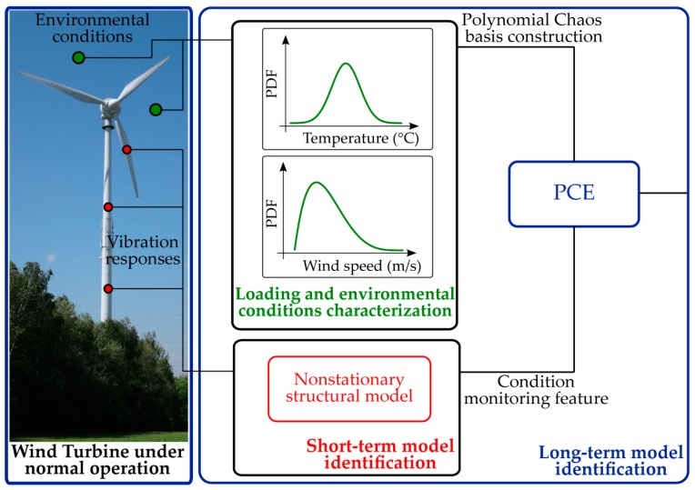
The complex dynamics of operational wind turbine (WT) structures challenges the applicability of existing structural health monitoring (SHM) strategies for condition assessment. At the center of Europe’s renewable energy strategic planning, WT systems call for implementation of strategies that may describe the WT behavior in its complete operational spectrum. The framework proposed in this paper relies on the symbiotic treatment of acting environmental/operational variables and the monitored vibration response of the structure. The approach aims at accurate simulation of the temporal variability characterizing the WT dynamics, and subsequently at the tracking of the evolution of this variability in a longer-term horizon. The bi-component analysis tool is applied on long-term data, collected as part of continuous monitoring campaigns on two actual operating WT structures located in different sites in Germany. The obtained data-driven structural models verify the potential of the proposed strategy for development of an automated SHM diagnostic tool.
Overview
The claims and statistics of this paper haven’t been checked yet.
Run the check — free, no account needed. It reads the open-access text and checks the sources it cites.
Integrity signals
Registry
Cites
Statistics
Figures
Verification
Claims the paper makes
The claims and statistics of this paper haven’t been checked yet.
Run the check — free, no account needed. It reads the open-access text and checks the sources it cites.
Claims other papers make about this one
Each is checked against this paper’s own text: does it say what the citing paper says it does?
The source backs part of the claim, not all of it — or backs it for a different population, condition or comparison.
In the citing paper
“Finally, perhaps the strongest case to be made for dependence of structural response on EOV is the case of wind turbine systems, where the EOV factors are logged in the form of statistical averages that are logged as supervisory control and data acquisition [33,34].”
From On the Consistent Classification and Treatment of Uncertainties in Structural Health Monitoring Applications (2025) · cites this paper as [33]
Experimental — accuracy not yet measured
Self-check
Percentages, sums and reported differences re-computed from the paper’s own numbers.
The self-check needs the paper’s full text.
Citations
Cites
Independent component analysis: algorithms and applications
Hyvärinen, A., & Erkki Oja, A. (2000) · Neural Networks · doi:10.1016/s0893-6080(00)00026-5 · Cited by 8,974
The Wiener--Askey Polynomial Chaos for Stochastic Differential Equations
Xiu, D., & Karniadakis, G. E. (2002) · SIAM Journal on Scientific Computing · doi:10.1137/s1064827501387826 · Cited by 4,807
Wiener, N. (1938) · American Journal of Mathematics · doi:10.2307/2371268 · Cited by 3,114
The Orthogonal Development of Non-Linear Functionals in Series of Fourier-Hermite Functionals
Cameron, R. H., & Martin, W. T. (1947) · Annals of Mathematics · doi:10.2307/1969178 · Cited by 1,290
Some basic hypergeometric orthogonal polynomials that generalize Jacobi polynomials
Askey, R., & Wilson, J. A. (1985) · Memoirs of the American Mathematical Society · doi:10.1090/memo/0319 · Cited by 1,154
Condition monitoring and fault detection of wind turbines and related algorithms: A review
Hameed, Z., Hong, Y., Cho, Y.-I., et al. (2007) · Renewable and Sustainable Energy Reviews · doi:10.1016/j.rser.2007.05.008 · Cited by 1,003
Spectral Methods for Uncertainty Quantification
Maître, O. P. L., & Knio, O. (2010) · Scientific computation · doi:10.1007/978-90-481-3520-2 · Cited by 953
Blatman, G., & Sudret, B. (2010) · Probabilistic Engineering Mechanics · doi:10.1016/j.probengmech.2009.10.003 · Cited by 832
Structural health monitoring for a wind turbine system: a review of damage detection methods
Ciang, C. C., Lee, J.-R., & Bang, H.-J. (2008) · Measurement Science and Technology · doi:10.1088/0957-0233/19/12/122001 · Cited by 802
Smoothness Priors Analysis of Time Series
Kitagawa, G., & Gersch, W. (1996) · Lecture notes in statistics · doi:10.1007/978-1-4612-0761-0 · Cited by 645
Research works printed but not linked: 6
- Oliveira, G., Magalhães, F., Cunha, Á., and Caetano, E. (2015, January 19–21). Automated modal tracking and fatigue assessment of a wind turbine based on continuous dynamic monitoring. Proceedings of the 6th International Conference on Experimental Vibration Analysis for Civil Engineering Structures (EVACES 2015), Dubendorf, Switzerland.
- Oliveira, G. (2016). Vibration-Based Structural Health Monitoring of Wind Turbines. [Ph.D. Thesis, University of Porto].
- Bogoevska, S., Spiridonakos, M., Chatzi, E., Dumova-Jovanoska, E., and Höffer, R. (2016, January 5–8). A novel bi-component structural health monitoring strategy for deriving global models of operational wind turbines. Proceedings of the 8th European Workshop on Structural Health Monitoring (EWSHM 2016), Bilbao, Spain.
- Ou, Y., Dertimanis, V., and Chatzi, E. (2016, January 19–21). Experimental Damage Detection of a wind turbine blade under varying operational conditions. Proceedings of the 5th International Conference on Uncertainty in Structural Dynamics (USD 2016), Leuven, Belgium.
- Lachmann, S., Baitsch, M., Hartmann, D., and Höffer, R. (2009, January 19–23). Structural lifetime prediction for wind energy converters based on health monitoring and system identification. Proceedings of the 5th European & African Conference on Wind Engineering (EACWE 2009), Florence, Italy.
- Oliveira, G., Magalhães, F., Cunha, Á., and Caetano, E. (2016, January 5–8). Optimization of a wind turbine vibration-based SHM system. Proceedings of the 8th European Workshop on Structural Health Monitoring (EWSHM 2016), Bilbao, Spain.
Cited by
Martín-Sanz, H., Tatsis, K., Dertimanis, V. K., Avendaño-Valencia, L. D., Brühwiler, E., & Chatzi, E. (2020) · Structure and Infrastructure Engineering · doi:10.1080/15732479.2019.1650079 · Cited by 22
Self-citationKamariotis, A., Vlachas, K., Ntertimanis, V., Koune, I., Cicirello, A., & Chatzi, E. (2025) · ASCE-ASME Journal of Risk and Uncertainty in Engineering Systems, Part B: Mechanical Engineering · doi:10.1115/1.4067140 · Cited by 15
Self-citation
Metadata
- Authors
- Bogoevska, S., Spiridonakos, M., Chatzi, E., Dumova-Jovanoska, E., & Höffer, R.
- Affiliations
- Faculty of Civil Engineering, University Ss. Cyril and Methodius, Skopje 1000, Macedonia
- Department of Civil, Environmental and Geomatic Engineering, ETH, Zürich CH-8093, Switzerland
- Department of Civil and Environmental Engineering, Ruhr-University Bochum, Bochum 44801, Germany
- ORCID
- Chatzi, Eleni
- Venue
- Sensors
- Publisher
- MDPI AG
- Published
- 2017-03-30
- Volume
- 17
- Issue
- 4
- Pages
- 720
- ISSN
- 1424-8220
- PMC
- PMC5421680
- Cited by
- 60
- References
- 36
- Language
- en
- Funders
- ERC (#67984 WINDMIL)
About these checks
Registry, retraction, Cites and statistics results are computed, not judged, with one exception: a printed reference that no index lists is read once by a model before it counts as a citation error. Claims are extracted by a model and kept only when their quote appears verbatim in the text; each cited source is then checked, with a model’s help, for whether it says what the claim relies on. Those verdicts can be wrong — read the claim’s quote and the cited source before relying on one.
Statistics and arithmetic are recomputed, not judged.
Confidence bands are shown only for fields calibrated on our annotated test set. None is calibrated yet, so no band is shown.
What counts as a claim ›How we measure confidence ›How we check this ›
Are you an author, or do you see a problem with this page? Request a review
How to cite
Cite CoChat for the checks on this page, and the paper for its own findings.
- This page
- CoChat. (2026). Citation check: A Data-Driven Diagnostic Framework for Wind Turbine Structures: A Holistic Approach. https://app.cochat.ai/papers/10.3390/s17040720
- The paper
- Bogoevska, S., Spiridonakos, M., Chatzi, E., Dumova-Jovanoska, E., & Höffer, R. (2017). A Data-Driven Diagnostic Framework for Wind Turbine Structures: A Holistic Approach. Sensors. https://doi.org/10.3390/s17040720
Data sources
Bibliographic data: Semantic Scholar, OpenAlex, Crossref.
Contains information from the Semantic Scholar Academic Graph Datasets, made available under the ODC Attribution License (ODC-BY 1.0).
Semantic Scholar’s data is described in: Kinney, R., et al. (2023). The Semantic Scholar Open Data Platform. arXiv:2301.10140.
