

Complex Deep Neural Networks from Large Scale Virtual IMU Data for Effective Human Activity Recognition Using Wearables
Open accessThe DOI matches its Crossref record; 48 of the 87 references it cites were found in a registry or an index, and 3 are not checked yet; 6 of the 50 sources its claims cite were checked for support.
Abstract
Supervised training of human activity recognition (HAR) systems based on body-worn inertial measurement units (IMUs) is often constrained by the typically rather small amounts of labeled sample data. Systems like IMUTube have been introduced that employ cross-modality transfer approaches to convert videos of activities of interest into virtual IMU data. We demonstrate for the first time how such large-scale virtual IMU datasets can be used to train HAR systems that are substantially more complex than the state-of-the-art. Complexity is thereby represented by the number of model parameters that can be trained robustly. Our models contain components that are dedicated to capture the essentials of IMU data as they are of relevance for activity recognition, which increased the number of trainable parameters by a factor of 1100 compared to state-of-the-art model architectures. We evaluate the new model architecture on the challenging task of analyzing free-weight gym exercises, specifically on classifying 13 dumbbell execises. We have collected around 41 h of virtual IMU data using IMUTube from exercise videos available from YouTube. The proposed model is trained with the large amount of virtual IMU data and calibrated with a mere 36 min of real IMU data. The trained model was evaluated on a real IMU dataset and we demonstrate the substantial performance improvements of 20% absolute F1 score compared to the state-of-the-art convolutional models in HAR.
Verified 2026-10-05 · 3 references not checked yet
Overview
CoChat Summary
TL;DR
The paper shows that large-scale virtual IMU data generated by IMUTube can train much more complex HAR models than previously feasible, using a model with about 1100× more trainable parameters than a standard ConvNet. On 13 dumbbell exercises, the best model reaches 80.2% mean F1, improving by 17.6 absolute points over a CNN baseline and 6.2 over DeepConvLSTM.
Key findings
- The proposed model trained with virtual IMU data achieved 80.2% mean F1, a +17.6% absolute improvement over the CNN baseline and +6.2% absolute over DeepConvLSTM.
- The full architecture contains approximately 1100× more trainable parameters than the convolutional baseline, with reported gains of 12.64% absolute F1 using real IMU only and 17.63% absolute F1 using real + virtual IMU.
- Adaptive trimming alone increased parameters by about 10× and improved F1 by 4.33% on average; multi-window kernels added another ~10× complexity and 3.44% absolute F1.
- Multi-view kernels gave 3.58% absolute F1 on average, skip connections 2.65% with virtual IMU, while recurrent layers and uncertainty modeling gave only marginal, non-significant improvements (0.19% and 0.27% absolute F1, respectively).
Methods
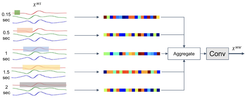
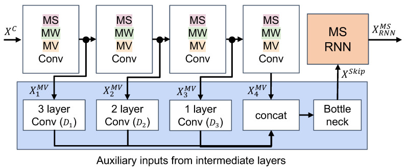
- The model combines adaptive sensor-window trimming, multi-scale hourglass convolutions, multi-window kernels, multi-view time-channel kernels, skip connections, multi-scale recurrent aggregation, and heteroscedastic uncertainty modeling for noisy samples.
- Virtual IMU data were generated with IMUTube from YouTube videos for 13 dumbbell exercises, yielding >41 h of virtual data; real IMU data came from MyoGym (10 users, 30 free-weight activities, 2.81 min per activity on average, about 36 min total for calibration).
- Evaluation used 30 Hz data, 4-second windows with 1-second overlap, subjects 1–5 for training, 6–7 for validation, 8–10 for testing, mean F1 score, and Wilson score intervals from 15 runs; models were pretrained on calibrated virtual IMU data and fine-tuned on real IMU data.
Limitations
- The paper states the virtual dataset is still relatively small compared with datasets like ImageNet, and that increasing virtual data may introduce noise that could counteract performance gains.
- The paper notes the studied gym exercises are relatively constrained, the architecture components were manually designed rather than learned via NAS, and uncertainty modeling had only marginal effect.
- Evident from the text: evaluation uses a single wrist sensor, 13 exercises, only 10 real users, weak labels from YouTube search terms, and a domain gap between virtual and real IMU data that requires calibration.
Model-written summary. Check it against the paper before relying on it.
Integrity signals
Registry
Cites
Statistics
Figures





Verification
Claims the paper makes
6 Valid · 7 Not valid · 27 Not checked · 75 Own results and interpretations
The cited sources support only part of this claim — read each source’s verdict below.
In the paper
“The popular DeepConvLSTM model [7] can only afford four, moderately-sized convolution layers to learn effective data representations, and two LSTM layers for sequence modeling.”
§ Complex Deep Neural Networks from Large Scale Virtual IMU Data for Effective Human Activity Recognition Using Wearables > 1. Introduction
What the sources say
- Partly supportedcites [7] Ordóñez F.J. Roggen D. Deep convolutional and lstm recurrent neural networks for multimodal wearable activity recognition Sensors 2016 16 115 10.3390/s16010115 26797612 PMC4732148 sourceExperimental — accuracy not yet measured
Section 3.1 (Architecture) confirms the structural part of the claim: DeepConvLSTM transforms sensor data 'through four convolutional operations' and adds two recurrent dense layers, shorthand 'C(64)-C(64)-C(64)-C(64)-R(128)-R(128)-Sm', with the two-layer recurrent depth chosen following prior work showing at least two recurrent layers beneficial. However, the 'can only afford' limitation is not what the source says: Section 5.4 (Discussion) states it is an eight-layer network while noting 'increasing further the number of layers may be beneficial', and Section 5.3 (Hyperparameters Evaluation, Figure 8) reports performance improving by ~1% per added convolutional layer on OPPORTUNITY. The paper frames the layer count as a deliberate trade-off with training time and computational budget, not a capacity the model cannot exceed. (LLM, conf=0.80)
plain- Asserted: passes — The authors put it forward as true.
- Checkable: passes — It can be checked against evidence.
- Load-bearing: passes — The paper’s conclusions depend on it.
- Based: passes — The paper gives a reason why it holds.
- Partly supported
The cited sources support only part of this claim — read each source’s verdict below.
In the paper
“The architectures of state-of-the-art HAR models, such as the DeepConvLSTM model [7], were designed specifically respecting the restrictions of limited size labeled training sets.”
§ Complex Deep Neural Networks from Large Scale Virtual IMU Data for Effective Human Activity Recognition Using Wearables > 1. Introduction
What the sources say
- Partly supportedcites [7] Ordóñez F.J. Roggen D. Deep convolutional and lstm recurrent neural networks for multimodal wearable activity recognition Sensors 2016 16 115 10.3390/s16010115 26797612 PMC4732148 sourceExperimental — accuracy not yet measured
Our copy supports only the small-labelled-data side of the claim: the Discussion (Section 5.4) observes that the recurrent model reaches very good performance on relatively small datasets (OPPORTUNITY, ~80 k sensor samples / 6 h of recordings) and that deep learning 'may actually be applicable to problem domains where acquiring annotated data is very costly, such as in supervised activity recognition' — a hedged post-hoc implication, not a stated design driver. The paper's actual stated design rationale (Abstract; Section 1 Introduction; Section 3 Architecture; Section 5.4) is automation of feature extraction to avoid engineered features and expert knowledge, explicit modelling of temporal dynamics, multimodal sensor fusion, a much reduced parameter count versus the fully-connected baseline CNN, and computational/training-time budget under the OPPORTUNITY sliding-window constraint; nowhere does it say the architecture was designed specifically to respect limited-size labeled training sets (drop-out is added as generic regularisation, Section 3.3, not tied to label scarcity). The generalisation to 'state-of-the-art HAR models' as a class is also not asserted in this source, which instead notes that convolution–recurrent combination had not yet been investigated in HAR (Section 2.3). (LLM, conf=0.72)
plainstates a cause- Asserted: passes — The authors put it forward as true.
- Checkable: passes — It can be checked against evidence.
- Load-bearing: passes — The paper’s conclusions depend on it.
- Based: passes — The paper gives a reason why it holds.
- Partly supported
The sources with a verdict support this claim; the rest weren’t checked yet, have no full text we could read, or their verdicts aren’t rated yet.
In the paper
“Recently, a paradigm change to data collection for supervised recognizer training has been introduced where existing repositories of videos of human activities are utilized to generate virtual IMU training data [14,15,16,17].”
§ Complex Deep Neural Networks from Large Scale Virtual IMU Data for Effective Human Activity Recognition Using Wearables > 1. Introduction
What the sources say
- Not checked yetcites [14] Kwon H. Tong C. Haresamudram H. Gao Y. Abowd G.D. Lane N.D. Ploetz T. IMUTube: Automatic extraction of virtual on-body accelerometry from video for human activity recognition Proc. ACM Interact. Mob. Wearable Ubiquitous Technol. 2020 4 1 29 10.1145/3411841 source
- Not checked yetcites [15] Kwon H. Wang B. Abowd G. Plötz T. Approaching the Real-World: Supporting Activity Recognition Training with Virtual IMU Data Proc. ACM Interact. Mob. Wearable Ubiquitous Technol. 2020 5 1 32 10.1145/3478096 source
- Supportedcites [16] Liu Y. Zhang S. Gowda M. When Video meets Inertial Sensors: Zero-shot Domain Adaptation for Finger Motion Analytics with Inertial Sensors Proceedings of the International Conference on Internet-of-Things Design and Implementation Charlottesville, VA, USA 18–21 May 2021 182 194 source
Section 2.1 (p. 3) says publicly available videos can be used to harvest training data and identifies a public sign-language tutorial as this paper’s source. Section 4 (p. 4) states that locations captured from video are transformed into synthetic accelerometer and orientation data for training ML models. (LLM, conf=0.94)
- Not checked yetcites [17] Rey V. Hevesi P. Kovalenko O. Lukowicz P. Let there be IMU data: Generating training data for wearable, motion sensor based activity recognition from monocular RGB videos Adjunct Proceedings of the ACM International Joint Conference on Pervasive and Ubiquitous Computing and Proceedings of the ACM International Symposium on Wearable Computers ACM New York, NY, USA 2019 699 708 source
plainstates a cause- Asserted: passes — The authors put it forward as true.
- Checkable: passes — It can be checked against evidence.
- Load-bearing: passes — The paper’s conclusions depend on it.
- Based: passes — The paper gives a reason why it holds.
The cited sources support only part of this claim — read each source’s verdict below.
In the paper
“Adding so-called skip-connections from intermediate layers directly to layers later in the model seemingly helps to counteract the vanishing gradient by preserving the flow of backpropagated gradient signals [86,87].”
§ Complex Deep Neural Networks from Large Scale Virtual IMU Data for Effective Human Activity Recognition Using Wearables > 3. Complex Deep Neural Networks for Human Activity Recognition > 3.4. Full Feature Extraction Model with Skip-Connection and Temporal Aggregation
What the sources say
- Not checked yetcites [86] He K. Zhang X. Ren S. Sun J. Deep residual learning for image recognition Proceedings of the IEEE Conference on Computer Vision and Pattern Recognition Las Vegas, NV, USA 27–30 June 2016 770 778 source
- Partly supportedcites [87] Szegedy C. Liu W. Jia Y. Sermanet P. Reed S. Anguelov D. Erhan D. Vanhoucke V. Rabinovich A. Going deeper with convolutions Proceedings of the IEEE Conference on Computer Vision and Pattern Recognition Boston, MA, USA 7–12 June 2015 1 9 sourceExperimental — accuracy not yet measured
Our copy of 'Going deeper with convolutions' supports only the gradient-flow half of the claim: Sec. 5 GoogLeNet (p. 6) states that, because effective gradient propagation through the 22-layer depth 'was a concern', adding auxiliary classifiers to intermediate layers (Inception 4a and 4d) was expected to 'increase the gradient signal that gets propagated back'. However, the paper's mechanism is side-branch auxiliary classifiers discarded at inference, not skip-connections routed from intermediate layers to later layers; no passage in our copy (searched: skip/shortcut connections, vanishing gradient, identity mapping) describes or uses skip connections, and the paper never uses the term 'vanishing gradient'. The skip-connection half of the attributed claim therefore rests on the other citation [86 or 87], not on this source. (LLM, conf=0.72)
hedgedstates a possible cause- Asserted: passes — The authors put it forward as true.
- Checkable: passes — It can be checked against evidence.
- Load-bearing: passes — The paper’s conclusions depend on it.
- Based: passes — The paper gives a reason why it holds.
The sources with a verdict support this claim; the rest weren’t checked yet, have no full text we could read, or their verdicts aren’t rated yet.
In the paper
“Previous work showed that training a large model is challenging because it becomes more likely that the gradient during optimization becomes infinitesimally small at the bottom layers [84,85,86].”
§ Complex Deep Neural Networks from Large Scale Virtual IMU Data for Effective Human Activity Recognition Using Wearables > 3. Complex Deep Neural Networks for Human Activity Recognition > 3.4. Full Feature Extraction Model with Skip-Connection and Temporal Aggregation
What the sources say
- Not checked yetcites [84] Hochreiter S. Bengio Y. Frasconi P. Schmidhuber J. Gradient Flow in Recurrent Nets: The Difficulty of Learning Long-Term Dependencies A Field Guide to Dynamical Recurrent Networks Kremer S.C. Kolen J.F. IEEE Press Piscataway, NJ, USA 2001 237 243
- Supportedcites [85] Goh G. Hodas N. Vishnu A. Deep learning for computational chemistry J. Comput. Chem. 2017 38 1291 1307 10.1002/jcc.24764 28272810 source
Section 2, “Deep Learning 101,” explains that error signals decay as they pass backward through multiple layers, calling this the vanishing gradient problem. It also says this problem made training deep networks difficult and practically capped their depth. (LLM, conf=0.90)
- Not checked yetcites [86] He K. Zhang X. Ren S. Sun J. Deep residual learning for image recognition Proceedings of the IEEE Conference on Computer Vision and Pattern Recognition Las Vegas, NV, USA 27–30 June 2016 770 778 source
hedgedstates a cause- Asserted: passes — The authors put it forward as true.
- Checkable: passes — It can be checked against evidence.
- Load-bearing: passes — The paper’s conclusions depend on it.
- Based: passes — The paper gives a reason why it holds.
60 more claims
Create a free account to see all 115 claims and to verify the 44 references still open.
- Probably not a substantial claim. 35
- It may state two separate claims as one. 19
- The quote only partly states this claim. 1
Claims other papers make about this one
Each is checked against this paper’s own text: does it say what the citing paper says it does?
The cited source says what the claim attributes to it.
In the citing paper
“The system leads to improving model performance when integrating real and virtual IMU data [108,109].”
From Past, Present, and Future of Sensor-based Human Activity Recognition Using Wearables: A Surveying Tutorial on a Still Challenging Task (2025) · cites this paper as [108]
The cited source says what the claim attributes to it.
In the citing paper
“Cross-modality transfer approaches [54,108,109,161,162] are instrumental for extracting virtual IMU data from 2D RGB videos of activities.”
From Past, Present, and Future of Sensor-based Human Activity Recognition Using Wearables: A Surveying Tutorial on a Still Challenging Task (2025) · cites this paper as [108]
Self-check
Percentages, sums and reported differences re-computed from the paper’s own numbers.
Each contradiction between two passages listed here was confirmed by an independent check.
Rated minor: it would not touch a result — a value no result rests on, a p-value that stays on the same side of the significance level, or a conflict that is clerical, resolved elsewhere in the paper, or outside its own findings.
In the paper
§ Complex Deep Neural Networks from Large Scale Virtual IMU Data for Effective Human Activity Recognition Using Wearables > 5. Discussion > 5.1. Collect Even Larger Datasets of Virtual IMU Data
“a total of approximately 41 hours, i.e., about 150,000 samples of 4-second data frames”
§ Complex Deep Neural Networks from Large Scale Virtual IMU Data for Effective Human Activity Recognition Using Wearables > 4. Case Study: Analyzing Free Weight Gym Exercises > 4.3. Evaluation Protocol
“we use a 4-second window with 1-second overlap across all experiments”
Citations
Cites
Deep Residual Learning for Image Recognition
He, K., Zhang, X., Ren, S., & Sun, J. (2016) · 2016 IEEE Conference on Computer Vision and Pattern Recognition (CVPR) · doi:10.1109/cvpr.2016.90 · Cited by 235,474 · cited 3×
“Previous work showed that training a large model is challenging because it becomes more likely that the gradient during optimization becomes infinitesimally small at the bottom layers [84–86].”
BackgroundMethodImageNet classification with deep convolutional neural networks
Krizhevsky, A., Sutskever, I., & Hinton, G. E. (2017) · Communications of the ACM · doi:10.1145/3065386 · Cited by 112,155 · cited 1×
“With such a massive dataset it is now possible to train very large models, such as the popular AlexNet [99], or ResNet-152 [86] that consists of 60 million trainable parameters.”
MethodHochreiter, S., & Schmidhuber, J. (1997) · Neural Computation · doi:10.1162/neco.1997.9.8.1735 · Cited by 102,318 · cited 1×
“Combined with recurrent neural network elements such as long short-term memory (LSTM) cells [27], effective models can be derived that capture both short-and long-term temporal dependencies by aggregating historical features along the sequence [7,25,26,28].”
BackgroundGoing deeper with convolutions
Szegedy, C., Liu, W., Jia, Y., Sermanet, P., Reed, S., Anguelov, D., Erhan, D., Vanhoucke, V., & Rabinovich, A. (2015) · 2015 IEEE Conference on Computer Vision and Pattern Recognition (CVPR) · doi:10.1109/cvpr.2015.7298594 · Cited by 48,562
ImageNet Large Scale Visual Recognition Challenge
Russakovsky, O., Deng, J., Su, H., Krause, J., Satheesh, S., Ma, S., Huang, Z., Karpathy, A., Khosla, A., Bernstein, M., et al. (2015) · International Journal of Computer Vision · doi:10.1007/s11263-015-0816-y · Cited by 39,380 · cited 1×
“For example, the popular ImageNet dataset consists of about 14 million annotated images [98], which is two orders of magnitude larger than our dataset.”
MethodLabaca-Castro, R. (2023) · Machine Learning under Malware Attack · doi:10.1007/978-3-658-40442-0_9 · Cited by 19,272
OpenPose: Realtime Multi-Person 2D Pose Estimation Using Part Affinity Fields
Cao, Z., Hidalgo, G., Simon, T., Wei, S.-E., & Sheikh, Y. (2021) · IEEE Transactions on Pattern Analysis and Machine Intelligence · doi:10.1109/tpami.2019.2929257 · Cited by 5,536 · cited 2×
“Standard multi-person 2D pose detectors often confuse people in a scene with non-human objects that may look like humans, which results in erroneous tracking [52].”
BackgroundProceedings European Conference on Computer Vision 2002
Heyden, A., Sparr, G., Nielsen, M., & Johansen, P. (2002) · Lund University Publications (Lund University) · Cited by 5,153
Jaderberg, M., Simonyan, K., Zisserman, A., & Kavukcuoglu, K. (2015) · arXiv · doi:10.48550/arxiv.1506.02025 · Cited by 5,137 · cited 1×
“The cropping operation, F crop ( X , s , e ) = F sampler ( F grid _ gen ( X ) , s , e ) , of AdapTrimm is fully differentiable, which is adapted from the grid generator, ´ X = F grid _ gen ( X ) , and sampler, F sampler ( ´ X , s , e ) , used in spatial transformer networks (STN) [71].”
BackgroundProbable Inference, the Law of Succession, and Statistical Inference
Wilson, E. B. (1927) · Journal of the American Statistical Association · doi:10.1080/01621459.1927.10502953 · Cited by 4,476 · cited 1×
“For the statistical significance test, Wilson score intervals are derived from 15 runs for each experiment [96].”
Method
Research works printed but not linked: 17
- Hammerla N.Y. Halloran S. Plötz T. Deep, Convolutional, and Recurrent Models for Human Activity Recognition Using Wearables AAAI Press Palo Alto, CA, USA 2016 1533 1540
- Fawaz H. Forestier G. Weber J. Idoumghar L. Muller P. Data augmentation using synthetic data for time series classification with deep residual networks arXiv 2018 1808.02455
- Ramponi G. Protopapas P. Brambilla M. Janssen R. T-cgan: Conditional generative adversarial network for data augmentation in noisy time series with irregular sampling arXiv 2018 1811.08295
- Yosinski J. Clune J. Bengio Y. Lipson H. How transferable are features in deep neural networks? arXiv 2014 1411.1792
- Vaswani A. Shazeer N. Parmar N. Uszkoreit J. Jones L. Gomez A.N. Kaiser L. Polosukhin I. Attention is all you need arXiv 2017 1706.03762
- Redmon J. Farhadi A. YOLOv3: An Incremental Improvement arXiv 2018 1804.02767
- Joel A. Stergios I. A Direct Least-Squares (DLS) method for PnP Proceedings of the 2011 International Conference on Computer Vision Barcelona, Spain 6–13 November 2011
- Vankadari M. Garg S. Majumder A. Kumar S. Behera A. Unsupervised monocular depth estimation for night-time images using adversarial domain feature adaptation Proceedings of the European Conference on Computer Vision Springer Cham, Switzerland 2020 443 459
- Kingma D. Ba J. Adam: A method for stochastic optimization arXiv 2014 1412.6980
- Li P. Lin Y. Schultz-Fellenz E. Contextual hourglass network for semantic segmentation of high resolution aerial imagery arXiv 2018 1810.12813
- Oñoro-Rubio D. Niepert M. Contextual Hourglass Networks for Segmentation and Density Estimation arXiv 2018 1806.04009
- Chung J. Ahn S. Bengio Y. Hierarchical multiscale recurrent neural networks arXiv 2016 1609.01704
- Kádár A. Côté M. Chrupała G. Alishahi A. Revisiting the hierarchical multiscale lstm arXiv 2018 1807.03595
- Kendall A. Gal Y. What uncertainties do we need in bayesian deep learning for computer vision? arXiv 2017 1703.04977
- Rolnick D. Veit A. Belongie S. Shavit N. Deep learning is robust to massive label noise arXiv 2017 1705.10694
- Misra I. Zitnick C.L. Hebert M. Shuffle and learn: Unsupervised learning using temporal order verification Proceedings of the European Conference on Computer Vision Springer Cham, Switzerland 2016 527 544
- Devlin J. Chang M. Lee K. Toutanova K. Bert: Pre-training of deep bidirectional transformers for language understanding arXiv 2018 1810.04805
Cited by
IMUGPT 2.0: Language-Based Cross Modality Transfer for Sensor-Based Human Activity Recognition
Leng, Z., Bhattacharjee, A., Rajasekhar, H., Zhang, L., Bruda, E., Kwon, H., & Plötz, T. (2024) · Proceedings of the ACM on Interactive, Mobile, Wearable and Ubiquitous Technologies · doi:10.1145/3678545 · Cited by 61
“Sensor-based human activity recognition using wearable devices (HAR), i.e., the automated assessment of what a person is doing (and when), has come a long way and it is considered one of the central pillars of mobile, wearable, and ubiquitous computing [36].”
InfluentialSelf-citationMekruksavanich, S., & Jitpattanakul, A. (2023) · Intelligent Automation & Soft Computing · doi:10.32604/iasc.2023.033542 · Cited by 45
Leng, Z., Kwon, H., & Ploetz, T. (2023) · Proceedings of the 2023 International Symposium on Wearable Computers · doi:10.1145/3594738.3611361 · Cited by 39
“Previous studies [10, 12] have shown that the extracted virtual IMU data lead to improved model performance when mixed with the real IMU data and allowed for effective training of more complex models.”
Self-citationHaresamudram, H., Tang, C. I., Suh, S., Lukowicz, P., & Plötz, T. (2025) · Proceedings of the ACM on Interactive Mobile Wearable and Ubiquitous Technologies · doi:10.1145/3729467 · Cited by 33
“Efforts to bridge the gap between video and Inertial Measurement Unit (IMU) data have gained prominence, with recent works addressing the challenge of translating video data into IMU representations [103, 104, 153, 154].”
InfluentialSelf-citationSignRing: Continuous American Sign Language Recognition Using IMU Rings and Virtual IMU Data
Li, J., Huang, L., Shah, S., Jones, S. J., Jin, Y., Wang, D., Russell, A., Choi, S., Gao, Y., Yuan, J., et al. (2023) · Proceedings of the ACM on Interactive Mobile Wearable and Ubiquitous Technologies · doi:10.1145/3610881 · Cited by 44
Synthetic Smartwatch IMU Data Generation from In-the-wild ASL Videos
Santhalingam, P. S., Pathak, P., Rangwala, H., & Kosecka, J. (2023) · Proceedings of the ACM on Interactive, Mobile, Wearable and Ubiquitous Technologies · doi:10.1145/3596261 · Cited by 28
Kwon, H., Clifford, G. D., Genias, I., Bernhard, D., Esper, C. D., Factor, S. A., & McKay, J. L. (2023) · Sensors · doi:10.3390/s23041766 · Cited by 24
“The model uses adaptive trimming (AT) to identify the core motion segment within each 4 s analysis window and trims the given input signal for further analysis [35].”
BackgroundMethodInfluentialSelf-citationXia, C., & Sugiura, Y. (2022) · Proceedings of the 2022 ACM International Symposium on Wearable Computers · doi:10.1145/3544794.3558460 · Cited by 22
“In addition to working on a 3D avatar to calculate the virtual IMU data, the deep end-to-end network can be designed to output the virtual IMU data directly from the imported 2D video [8, 10, 24].”
BackgroundPhysical human locomotion prediction using manifold regularization
Javeed, M., Shorfuzzaman, M., Alsufyani, N., Chelloug, S. A., Jalal, A., & Park, J. (2022) · PeerJ Computer Science · doi:10.7717/peerj-cs.1105 · Cited by 18
If only we had more data!: Sensor-Based Human Activity Recognition in Challenging Scenarios
Plötz, T. (2023) · 2023 IEEE International Conference on Pervasive Computing and Communications Workshops and other Affiliated Events (PerCom Workshops) · doi:10.1109/percomworkshops56833.2023.10150267 · Cited by 16
“Our IMUTube system [53], [59], [60] (illustrated in Fig.”
MethodSelf-citationKwon, M. P., Hullfish, T. J., Humbyrd, C. J., Boakye, L. A. T., & Baxter, J. R. (2023) · Scientific Reports · doi:10.1038/s41598-023-45375-x · Cited by 14
Uhlenberg, L., Haeusler, L. O., & Amft, O. (2024) · IEEE Access · doi:10.1109/access.2024.3513477 · Cited by 16
“Similar observations in the literature confirm that mixing synthetic and measured data generally offers better possibilities to improve model performance compared to using only synthetic data or no augmentation [18], [20], [21], [27], [69].”
MuJo: Multimodal Joint Feature Space Learning for Human Activity Recognition
Fritsch, S. G., Oguz, C., Rey, V. F., Ray, L. S. S., Kiefer-Emmanouilidis, M., & Lukowicz, P. (2025) · IEEE International Conference on Pervasive Computing and Communications · doi:10.1109/percom64205.2025.00020 · Cited by 16
“Those chapters are manually added by the uploader or automatically generated.”
Semi-Supervised Adversarial Auto-Encoder to Expedite Human Activity Recognition
Thapa, K., Seo, Y., Yang, S., & Kim, K. (2023) · Sensors · doi:10.3390/s23020683 · Cited by 13
“By learning to extract features from raw sensor data automatically, deep learning approaches, such as LSTM [26], CNN [27], convLSTM [28], and CNN-LSTM [29] have demonstrated impressive improvements in performance compared to their shallow counterparts.”
On the Utility of Virtual On-body Acceleration Data for Fine-grained Human Activity Recognition
Leng, Z., Jain, Y., Kwon, H., & Plötz, T. (2023) · International Symposium on Wearable Computers · doi:10.1145/3594738.3611364 · Cited by 13
“IMUTube was mainly designed, deployed, and validated for human activities with underlying coarse motions, such as locomotion or gym exercises [17, 19].”
Self-citationLim, J., Luo, C., Lee, S., Song, Y. E., & Jung, H. (2024) · Sensors · doi:10.3390/s24082595 · Cited by 14
“…learning techniques to process raw IMU data for action classification, including recurrent neural networks (RNNs) [35], LSTM networks [36], CNNs [37], and hybrid CNN-LSTM models [38], showcasing the potential of IMU sensors in overcoming the challenges posed by vision-based action recognition…”
BackgroundMoghaddam, E. S., Ellis, C., & Hejrati, B. (2025) · IEEE Access · doi:10.1109/access.2025.3606339 · Cited by 6
“These models are successful in capturing the temporal dynamics of human activities [26], [27].”
Guan, L., Zhang, X., Cong, X., Zhang, Z., Yang, Z., Li, N., & Noureldin, A. M. (2024) · Measurement · doi:10.1016/j.measurement.2024.115682 · Cited by 6
Kanoga, S., Tsukiji, Y., & Karakida, R. (2025) · Expert Systems with Applications · doi:10.1016/j.eswa.2025.127469 · Cited by 5
Exercise Classification in Resistance Training: A Systematic Review of Technological Approaches
Brennan, T. R., Weakley, J. J. S., Johnston, R. D., & Creaby, M. W. (2025) · Sports Medicine · doi:10.1007/s40279-025-02281-8 · Cited by 2
SensorGPT: A New Paradigm for Synthetic Sensory Data Generation
Sharma, R., Khamis, A., Khalifa, S., Bretherton, D., & Kusý, B. (2025) · IEEE International Conference on Pervasive Computing and Communications Workshops (PerCom Workshops) · doi:10.1109/percomworkshops65533.2025.00061 · Cited by 2
“Existing cross-modality transfer ( dataset recycling ) approaches [10]–[12] use a mapping function to transform source context, such as a dataset or simulation, into synthetic target data.”
Wang, Q., & Xia, C. (2025) · International Conference on Cyberworlds (CW) · doi:10.1109/cw68232.2025.00058 · Cited by 1
“Hybrid training strategies combining virtual and real data [12], [13] alleviate this issue but often require extensive fine-tuning of the entire model, limiting deployment flexibility and increasing computational cost.”
Wei, M., Zhao, J. W. A. W., Sun, D., Zhang, J., Li, S., & Zhang, T. (2026) · IEEE Transactions on Instrumentation and Measurement · doi:10.1109/tim.2026.3667343 · Cited by 1
“M OTION capture technology [1] is widely applied in virtual reality [2], motor rehabilitation [3], [4], and sports analysis [5], [6], [7], [8], [9].”
Haresamudram, H., Tang, C. I., Suh, S., Lukowicz, P., & Ploetz, T. (2024) · arXiv · Cited by 31
“Efforts to bridge the gap between video and Inertial Measurement Unit (IMU) data have gained prominence, with recent works addressing the challenge of translating video data into IMU representations [103, 104, 153, 154].”
InfluentialSelf-citationEfficient Human Activity Recognition Based on Grouped Representations of Multimodal Wearable Data
Habault, G., & Wada, S. (2023) · Lecture notes of the Institute for Computer Sciences, Social Informatics and Telecommunications Engineering · doi:10.1007/978-3-031-33614-0_16
Synthetic Sensory Data Generators: How Much Progress Are We Making?
Sharma, R., Khamis, A., Khalifa, S., Bretherton, D., & Kusý, B. (2025) · IEEE International Conference on Pervasive Computing and Communications Workshops (PerCom Workshops) · doi:10.1109/percomworkshops65533.2025.00084 · Cited by 1
“Previous studies on sensory data synthesis have utilised cross-modality transfer ( dataset recycling ) approaches [6], [8]– [10] to convert data from one modality, such as 2D RGB videos of human activities, to another modality like IMU data.”
Adapting and Evaluating Human Motion Models for Generating Synthetic Gesture Sensor Data
Kalyani, P., Espinoza, A. A., & Longoria, R. G. (2025) · IFAC-PapersOnLine · doi:10.1016/j.ifacol.2025.12.214
Tiny but Mighty: When Smart Rings Meet Large Language Models
Olapade, M., Akintola, A., Yin, Z., Kuchida, R., Radeta, M., & Flores, H. (2025) · ACM International Joint Conference on Pervasive and Ubiquitous Computing (UbiComp) · doi:10.1145/3714394.3756295 · Cited by 1
“Moreover, ongoing miniaturization of IMUs has enabled their integration into compact wearables like smartwatches[15], smart rings [19], ear-buds [8], and fitness bands [26], making them suitable for capturing fine-grained, gesture-level activities such as hand gestures, finger taps, and brushing…”
A Quantitative Comparison of Human Body Modeling Methods to Synthesize IMU Data
Uhlenberg, L., Kempfle, J., Haeusler, L. O., & Amft, O. (2026) · IEEE Access · doi:10.1109/access.2026.3726408
“Kwon et al. [25], [26], [27] introduced IMUTube, which converts online video recordings into inertial data by using a 3D pose estimation model (VideoPose3D [28]) to track individual joints.”
Gu, Z., Yang, R., Shi, Y., Dai, D., Li, C., Huang, B., Jiao, K., Tao, Y., Wen, Y., Zhong, Y., et al. (2026) · Sensors · doi:10.3390/s26185838
Role of Language-Derived Semantics in Knowledge Distillation on Wearable Sensor Data
Kang, M. C., Jeong, J. C., Turaga, P. K., & Jeon, E. S. (2026) · Biomimetics · doi:10.3390/biomimetics11100729
“Although adding such layers and modules can improve model performance, it inevitably increases model complexity and computational costs [26], making these approaches less suitable for resource-constrained devices commonly used for wearable sensor data analysis.”
Metadata
- Authors
- Kwon, H., Abowd, G. D., & Plötz, T.
- Affiliations
- Georgia Institute of Technology (US)
- Northeastern University (US)
- Corresponding author
- Plötz, Thomas
- Venue
- Sensors
- Publisher
- MDPI AG
- Published
- 2021-12-13
- Volume
- 21
- Issue
- 24
- Pages
- 8337
- ISSN
- 1424-8220 (ISSN-L)
- PMC
- PMC8707382
- OpenAlex
- W4200504110
- Cited by
- 30
- References
- 86
- Citations by year
- 2026: 4 · 2025: 10 · 2024: 4 · 2023: 10 · 2022: 2
- FWCI
- 1.44
- Type
- journal article
- Language
- en
- Open access
- gold
- doi.org
- Licence
- Locations
- Sensors (publishedVersion, cc-by)
- PubMed Central (publishedVersion, cc-by)
- PubMed (publishedVersion)
- DOAJ (DOAJ: Directory of Open Access Journals) (submittedVersion, cc-by-sa)
- Funders
- Samsung Scholarship Program (N/A)
- Oracle for Research (N/A)
- Topics
- Physical Sciences › Computer Science › Computer Vision and Pattern Recognition › Context-Aware Activity Recognition Systems
- Physical Sciences › Computer Science › Computer Vision and Pattern Recognition › Human Pose and Action Recognition
- Physical Sciences › Engineering › Biomedical Engineering › Gait Recognition and Analysis
- Keywords
- human activity recognition, inertial measurement unit, wearable sensors, cross-modality transfer, deep neural network, model complexity, dumbbell exercise, transfer learning
- MeSH terms
- Wearable Electronic Devices, Humans, Human Activities, Neural Networks, Computer, Recognition, Psychology
About these checks
Registry, retraction, Cites and statistics results are computed, not judged, with one exception: a printed reference that no index lists is read once by a model before it counts as a citation error. Claims are extracted by a model and kept only when their quote appears verbatim in the text; each cited source is then checked, with a model’s help, for whether it says what the claim relies on. Those verdicts can be wrong — read the claim’s quote and the cited source before relying on one.
The claim verdicts this report counts are experimental: their accuracy is not yet measured.
A language model drew the claims from the paper on 2026-10-05, under version 3 of the claim definition (model deepseek-v4.1-flash, prompt extract-v3).
A second model labelled each claim on 2026-10-05 (model jev-1.13-20260917, definition revision gold-guideline-v0.2).
Cited sources are checked with a language model’s help (qwen3.8-omni-flash and gpt-6-sol).
Statistics and arithmetic are recomputed, not judged.
Confidence bands are shown only for fields calibrated on our annotated test set. None is calibrated yet, so no band is shown.
What counts as a claim ›How we measure confidence ›How we check this ›
Are you an author, or do you see a problem with this page? Request a review
Data sources
Bibliographic data: Semantic Scholar, OpenAlex, Crossref.
Contains information from the Semantic Scholar Academic Graph Datasets, made available under the ODC Attribution License (ODC-BY 1.0).
Semantic Scholar’s data is described in: Kinney, R., et al. (2023). The Semantic Scholar Open Data Platform. arXiv:2301.10140.
