

The DOI matches its DataCite record; 34 of the 34 references it cites were found in a registry or an index; none of the 34 sources its claims cite is checked for support yet.
AlphaEarth Foundations: An embedding field model for accurate and efficient global mapping from sparse label data
Open accessAbstract
Unprecedented volumes of Earth observation data are continually collected around the world, but high-quality labels remain scarce given the effort required to make physical measurements and observations. This has led to considerable investment in bespoke modeling efforts translating sparse labels into maps. Here we introduce AlphaEarth Foundations, an embedding field model yielding a highly general, geospatial representation that assimilates spatial, temporal, and measurement contexts across multiple sources, enabling accurate and efficient production of maps and monitoring systems from local to global scales. The embeddings generated by AlphaEarth Foundations are the only to consistently outperform a suite of other well-known/widely accepted featurization approaches tested on a diverse set of mapping evaluations without re-training. We have released a dataset of global, annual, analysis-ready embedding field layers from 2017 through 2024.
Overview
AI snapshot
Written from the paper’s full text.
TL;DR
AlphaEarth Foundations (AEF) is a geospatial embedding field model that assimilates multi-source Earth observation data into a 64-byte, 10-meter representation and consistently outperforms designed and learned featurization baselines across sparse-label mapping evaluations. The authors release global annual embedding field layers from 2017 through 2024 and an evaluation suite.
Key findings
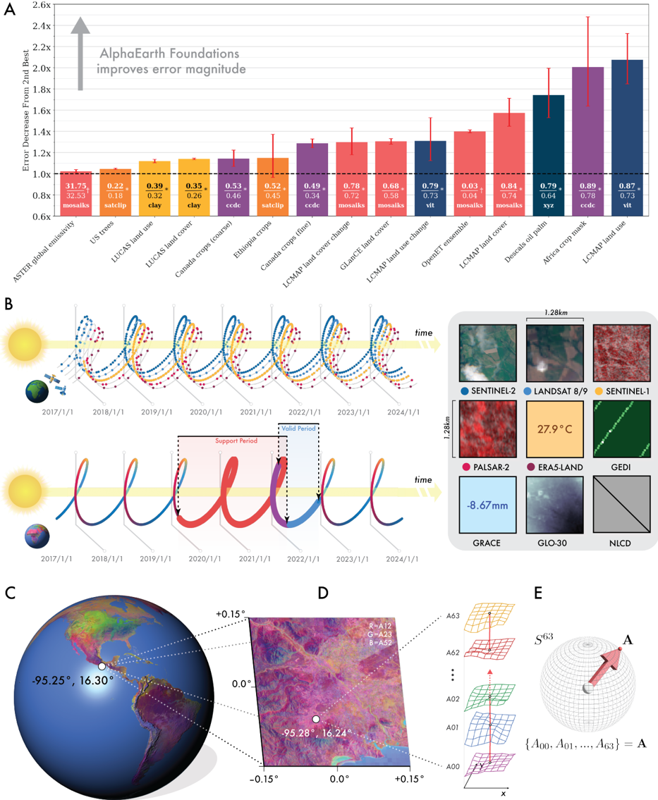
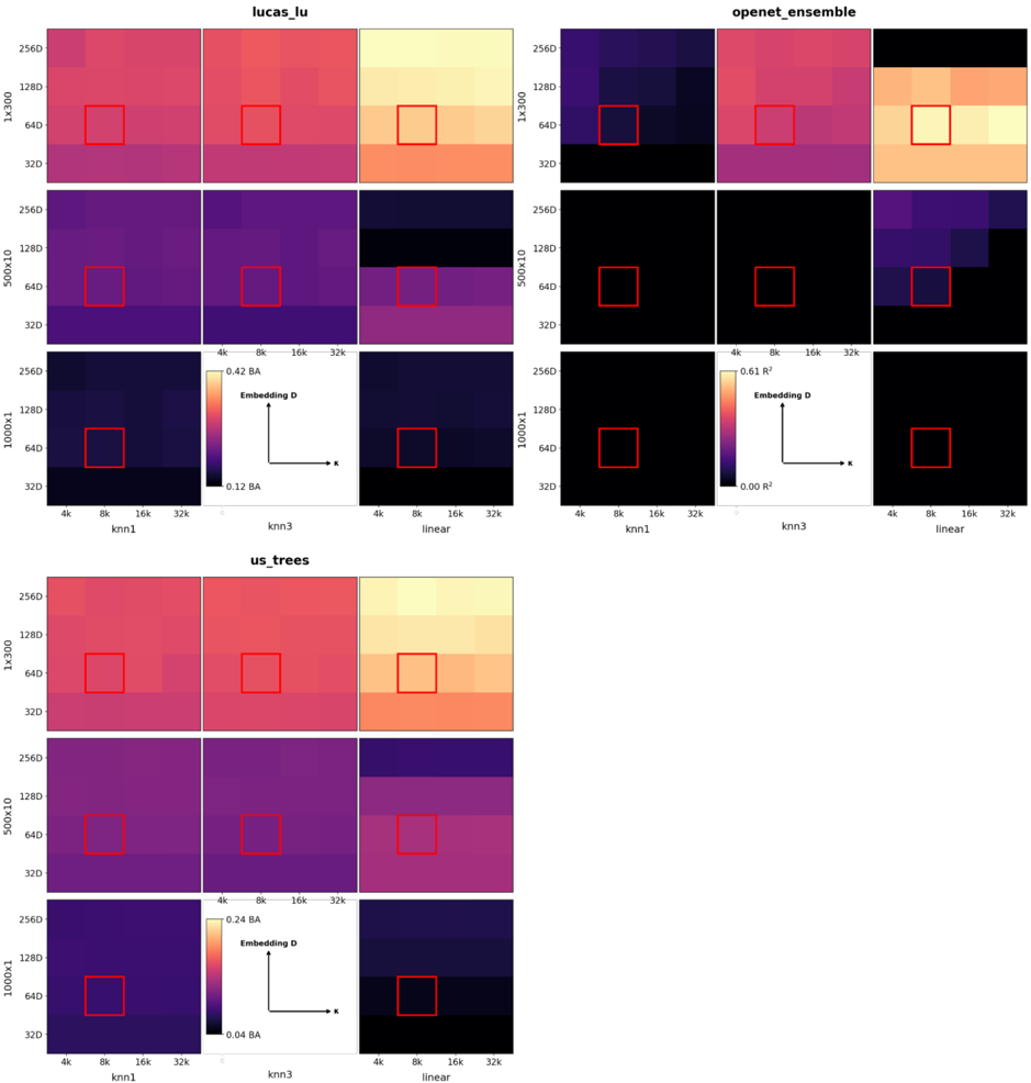
- AEF reduced error magnitudes by ∼23.9% on average versus the next-best approach/method of transfer in the max-trial setting, ∼10.4% in ten-shot trials, and ∼4.18% in one-shot trials across 15 evaluations sourced from 11 openly available datasets.
- AEF maintains 10-meter spatial resolution and requires 16x less information per representation (64 bytes) compared to the next-most compact learned method.
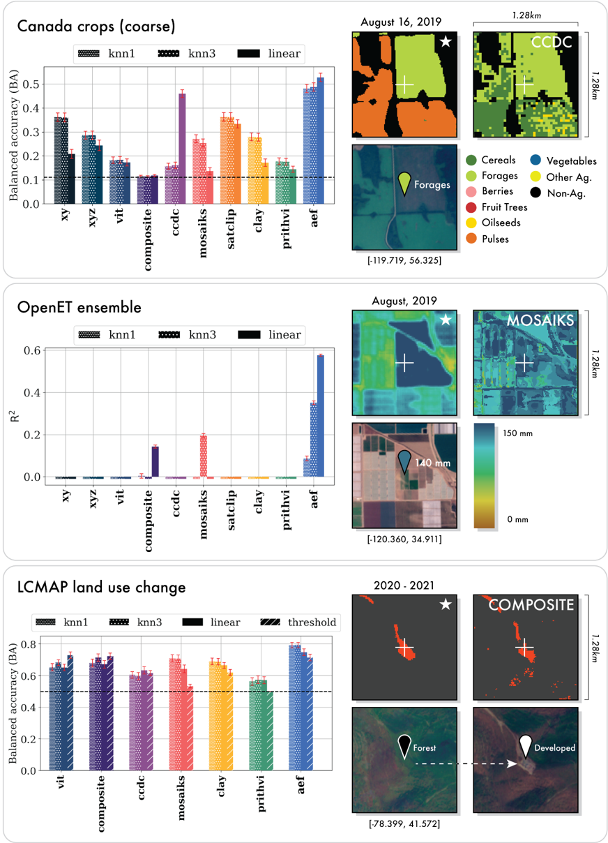
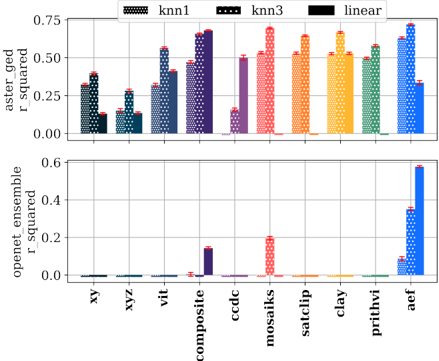
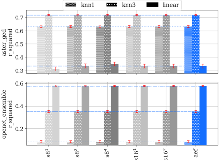
- For biophysical variables, AEF had the highest emissivity R² (0.72 ± 0.00) versus MOSAIKS (0.69 ± 0.00), and was the only method with R² > 0.2 for evapotranspiration, achieving R² = 0.58 ± 0.01.
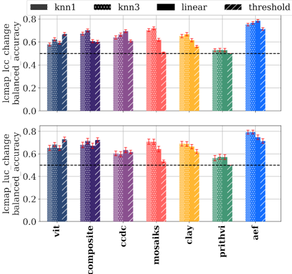
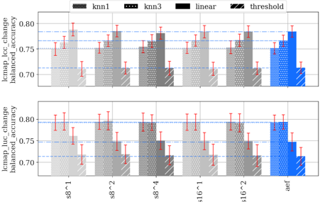
- In change detection with direct supervision, AEF achieved 78.4% ± 1.11 balanced accuracy (linear) for land cover and 79.3% ± 1.67 BA (kNN, k=3) for land use, versus next-best 72.0% ± 1.28 BA (MOSAIKS, kNN, k=3) and 71.5% ± 2.33 BA (composite, kNN, k=3), respectively.
Methods
- AEF was trained on over 3 billion observations across nine gridded data sources and one unstructured text source, representing approximately 1.1% of Earth’s land surface; training used 8,412,511 video sequences, 3,047,520,515 frames, and 5,145,244 sites, for 56 hours on 512 TPU v4 devices over 100k steps in batches of 256 video sequences.
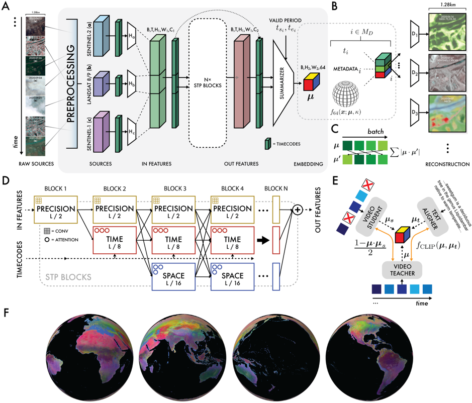
- The model uses a Space Time Precision (STP) encoder with simultaneous space, time, and precision operators, implicit decoders conditioned on time and sensor metadata, a von Mises-Fisher bottleneck in S⁶³, batch uniformity, teacher-student consistency, and text-contrastive learning with a frozen language model.
- Evaluation used 15 datasets derived from 11 openly available sources, with low-shot trials of n = 1, 10, and max samples per class, k-nearest neighbors and linear transfer methods, and comparisons against CCDC, MOSAIKS, composites, SatCLIP, Prithvi, Clay, and XY/XYZ/ViT controls.
Limitations
- The paper states that extreme low-shot performance remains unsolved: for 10-shot trials, AEF error reductions were > 1.0x in the ∼90% confidence interval for only 8/15 evaluations (average variation ±0.38x), and for 1-shot trials only 5/15 evaluations (average variation ±0.49x).
- The paper states that tile artifacts are still visible in embedding field layers due to irregular inputs and could be removed in future work with a more aggressive consistency objective; it also notes that US trees required ∼100x more observations than SatCLIP, speculated to relate to AEF receiving no coordinate information.
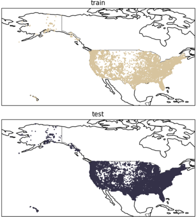
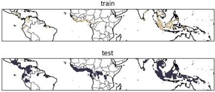
- The paper states that training locations inherit sampling biases from GBIF and Wikipedia, tending to cluster in denser human populations/urbanized areas; the text also makes evident that several evaluations are proxy tasks based on model-generated products (e.g., OpenET ensemble, ASTER GED) and that results reflect AEF v2.0, with v2.1 fixes described separately.
Model-written summary. Check it against the paper before relying on it.
Integrity signals
Registry
Cites
Statistics
Figures
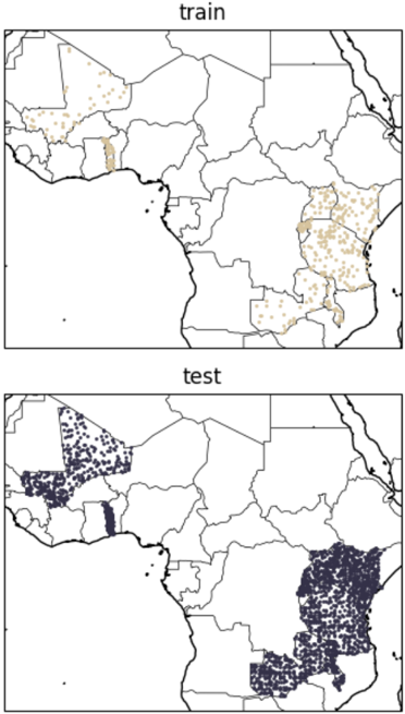
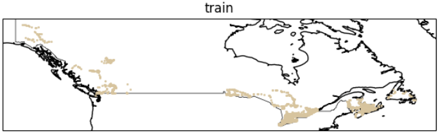
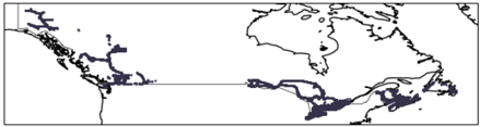
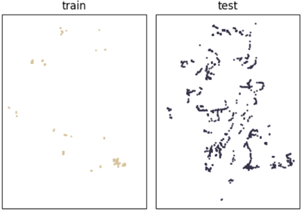
Verification
Claims the paper makes
64 Own result · 41 Own interpretation · 31 No basis given · 26 Own method · 21 Sources not found · 3 Not checked yet
A result the paper reports from its own data — it cites no other source for it, so there is none to check. The quote shows it is in the paper.
In the paper
“reducing error magnitudes by ∼23.9% (∼1.4x error magnitude reduction) on average”
- Also stated in: § Evaluation in realistic data-scarce scenarios · plain
“AEF reduced error magnitudes overall by ∼23.9% on average when compared to the next-best approach and method of transfer in the max-trial setting (Figure 1A).”
§ AlphaEarth Foundations: An embedding field model for accurate and efficient global mapping from sparse label data > AlphaEarth Foundations
plaindirect- Asserted: passes — The authors put it forward as true.
- Checkable: passes — It can be checked against evidence.
- Load-bearing: passes — The paper’s conclusions depend on it.
- Based: passes — The paper gives a reason why it holds.
- Also stated in: § Evaluation in realistic data-scarce scenarios · plain
A result the paper reports from its own data — it cites no other source for it, so there is none to check. The quote shows it is in the paper.
In the paper
“The embeddings generated by AlphaEarth Foundations are the only to consistently outperform a suite of other well-known/widely accepted featurization approaches tested on a diverse set of mapping evaluations without re-training.”
- Also stated in: § Introduction · plain
“The features produced by our model consistently achieve top performance in all application domains tested when compared to other general and even domain specific approaches (Figure 1A).”
- Also stated in: § Evaluation in realistic data-scarce scenarios · plain
“Our evaluations showed AEF consistently outperforms both designed and learned featurization methods in all trial settings.”
§ AlphaEarth Foundations: An embedding field model for accurate and efficient global mapping from sparse label data > Abstract
boosteddirect- Asserted: passes — The authors put it forward as true.
- Checkable: passes — It can be checked against evidence.
- Load-bearing: passes — The paper’s conclusions depend on it.
- Based: passes — The paper gives a reason why it holds.
- Also stated in: § Introduction · plain
The paper states this without a source or data behind it here, so there is nothing to check it against. The quote shows it is in the paper.
In the paper
“while maintaining a best-in-class 10-meter spatial resolution”
§ AlphaEarth Foundations: An embedding field model for accurate and efficient global mapping from sparse label data > AlphaEarth Foundations
plain- Asserted: passes — The authors put it forward as true.
- Checkable: passes — It can be checked against evidence.
- Load-bearing: passes — The paper’s conclusions depend on it.
- Based: passes — The paper gives a reason why it holds.
The paper states this without a source or data behind it here, so there is nothing to check it against. The quote shows it is in the paper.
In the paper
“Critically, as we will show, existing learned featurization approaches don't always outperform designed featurization methods in scarce data regimes.”
§ AlphaEarth Foundations: An embedding field model for accurate and efficient global mapping from sparse label data > From sparse labels to maps
plain- Asserted: passes — The authors put it forward as true.
- Checkable: passes — It can be checked against evidence.
- Load-bearing: passes — The paper’s conclusions depend on it.
- Based: unclear — It is unclear why the paper says it holds.
A result the paper reports from its own data — it cites no other source for it, so there is none to check. The quote shows it is in the paper.
In the paper
“In our extreme low-shot trials, overall performance of methods was close to random chance in many cases.”
§ AlphaEarth Foundations: An embedding field model for accurate and efficient global mapping from sparse label data > S6.1. Comparisons with 10 and 1 samples perclass
plain- Asserted: passes — The authors put it forward as true.
- Checkable: passes — It can be checked against evidence.
- Load-bearing: passes — The paper’s conclusions depend on it.
- Based: passes — The paper gives a reason why it holds.
A result the paper reports from its own data — it cites no other source for it, so there is none to check. The quote shows it is in the paper.
In the paper
“In the maxtrial setting, we find that all baselines were able to explain emissivity for some method of transfer with 𝑅 2 > 0.5 except for xy, xyz, and CCDC.”
§ AlphaEarth Foundations: An embedding field model for accurate and efficient global mapping from sparse label data > Estimating biophysical variables
plaincorrelational- Asserted: passes — The authors put it forward as true.
- Checkable: passes — It can be checked against evidence.
- Load-bearing: unclear — It is unclear whether the paper’s conclusions depend on it.
- Based: passes — The paper gives a reason why it holds.
The paper states this without a source or data behind it here, so there is nothing to check it against. The quote shows it is in the paper.
In the paper
“that requires 16x less information per-representation (64 bytes) compared to the next-most compact learned method”
§ AlphaEarth Foundations: An embedding field model for accurate and efficient global mapping from sparse label data > AlphaEarth Foundations
plain- Asserted: passes — The authors put it forward as true.
- Checkable: passes — It can be checked against evidence.
- Load-bearing: passes — The paper’s conclusions depend on it.
- Based: passes — The paper gives a reason why it holds.
A result the paper reports from its own data — it cites no other source for it, so there is none to check. The quote shows it is in the paper.
In the paper
“We found the version described here the most performant.”
§ AlphaEarth Foundations: An embedding field model for accurate and efficient global mapping from sparse label data > S5.2.1. Composites
plain- Asserted: passes — The authors put it forward as true.
- Checkable: passes — It can be checked against evidence.
- Load-bearing: unclear — It is unclear whether the paper’s conclusions depend on it.
- Based: passes — The paper gives a reason why it holds.
A result the paper reports from its own data — it cites no other source for it, so there is none to check. The quote shows it is in the paper.
In the paper
“For ten-shot trials, AEF reduced error magnitudes by ∼10.4% on average compared to the next-best approach”
§ AlphaEarth Foundations: An embedding field model for accurate and efficient global mapping from sparse label data > Evaluation in realistic data-scarce scenarios
plaindirect- Asserted: passes — The authors put it forward as true.
- Checkable: passes — It can be checked against evidence.
- Load-bearing: passes — The paper’s conclusions depend on it.
- Based: passes — The paper gives a reason why it holds.
A result the paper reports from its own data — it cites no other source for it, so there is none to check. The quote shows it is in the paper.
In the paper
“For the applications considered, AEF often offers a notable improvement over other archetypal examples of other designed and learned feature spaces.”
§ AlphaEarth Foundations: An embedding field model for accurate and efficient global mapping from sparse label data > S6.2. Classification
plaindirect- Asserted: passes — The authors put it forward as true.
- Checkable: passes — It can be checked against evidence.
- Load-bearing: passes — The paper’s conclusions depend on it.
- Based: passes — The paper gives a reason why it holds.
- Probably not a substantial claim. 64
- It may state two separate claims as one. 63
- The quote only partly states this claim. 2
The paper states this without a source or data behind it here, so there is nothing to check it against. The quote shows it is in the paper.
In the paper
“We note that AEF demonstrates improved spatial coherence without loss of spatial precision.”
§ AlphaEarth Foundations: An embedding field model for accurate and efficient global mapping from sparse label data > Thematic mapping
boosteddirect- Asserted: passes — The authors put it forward as true.
- Checkable: passes — It can be checked against evidence.
- Load-bearing: fails — The paper’s conclusions may not depend on it.
- Based: fails — The paper may give no reason why it holds.
Probably not a substantial claim. The paper’s conclusions may not depend on it. The paper may give no reason why it holds. It may state two separate claims as one.
A result the paper reports from its own data — it cites no other source for it, so there is none to check. The quote shows it is in the paper.
In the paper
“and for one-shot trials AEF reduced error magnitudes by ∼4.18%.”
§ AlphaEarth Foundations: An embedding field model for accurate and efficient global mapping from sparse label data > Evaluation in realistic data-scarce scenarios
plaindirect- Asserted: passes — The authors put it forward as true.
- Checkable: passes — It can be checked against evidence.
- Load-bearing: passes — The paper’s conclusions depend on it.
- Based: passes — The paper gives a reason why it holds.
The quote only partly states this claim.
The paper states this without a source or data behind it here, so there is nothing to check it against. The quote shows it is in the paper.
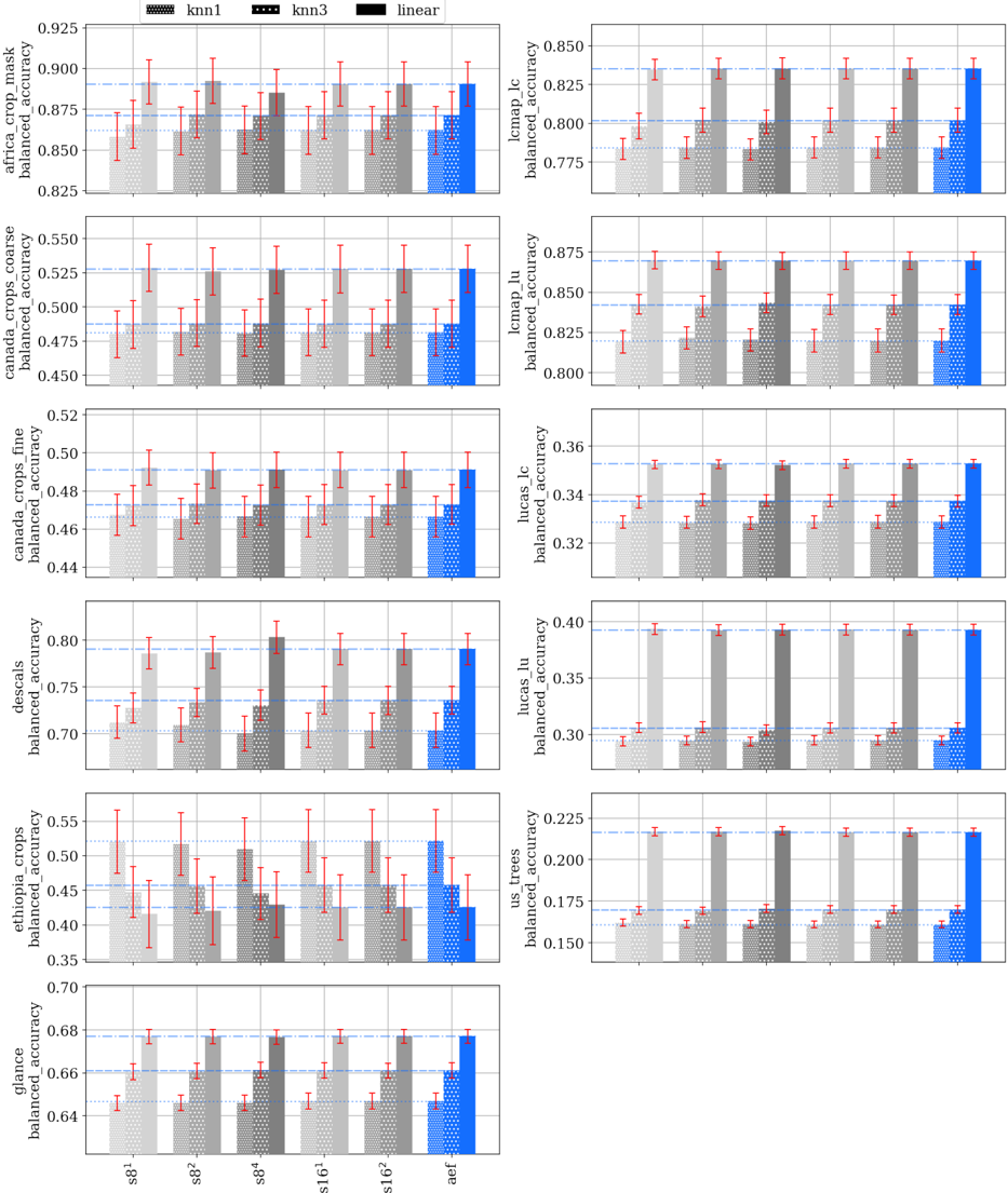
In the paper
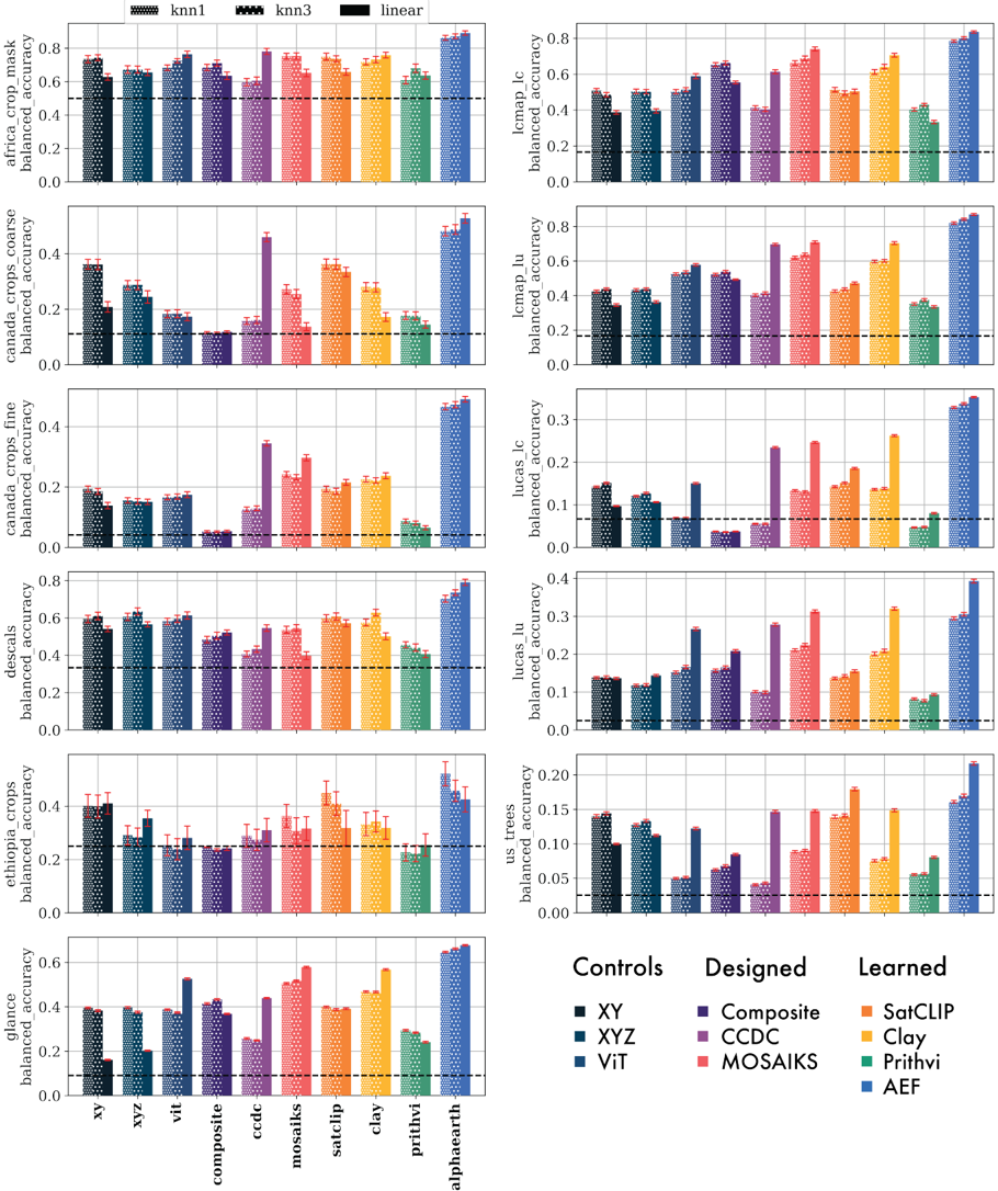
“We find that MOSAIKS is the next-best predictor for GLancE and LCMAP land cover, while Clay for LUCAS land use and land cover.”
§ AlphaEarth Foundations: An embedding field model for accurate and efficient global mapping from sparse label data > S6.2. Classification
plaincorrelational- Asserted: passes — The authors put it forward as true.
- Checkable: passes — It can be checked against evidence.
- Load-bearing: passes — The paper’s conclusions depend on it.
- Based: passes — The paper gives a reason why it holds.
It may state two separate claims as one.
A result the paper reports from its own data — it cites no other source for it, so there is none to check. The quote shows it is in the paper.
In the paper
“LUCAS land cover max-trial linear transfer BA scores were ~34.7% for 𝑏 = 0.005 and ~34.2% for 𝑏 = 0.”
§ AlphaEarth Foundations: An embedding field model for accurate and efficient global mapping from sparse label data > S2.2.4. Batch uniformity objective
plain- Asserted: passes — The authors put it forward as true.
- Checkable: passes — It can be checked against evidence.
- Load-bearing: unclear — It is unclear whether the paper’s conclusions depend on it.
- Based: passes — The paper gives a reason why it holds.
It may state two separate claims as one.
A result the paper reports from its own data — it cites no other source for it, so there is none to check. The quote shows it is in the paper.
In the paper
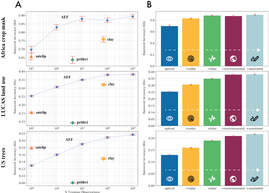
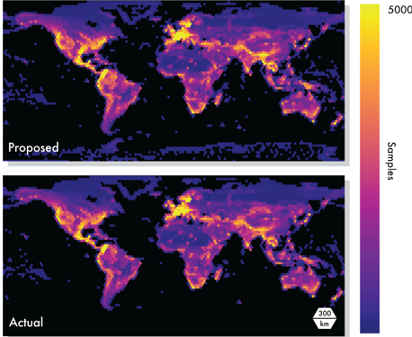
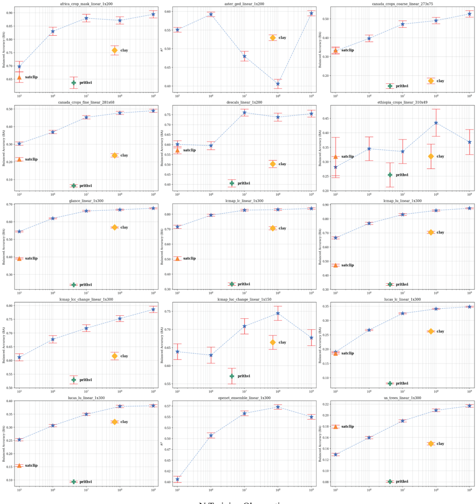
“For some evaluations (LUCAS land use, Africa crop mask), performance saturated between 100 million and 1 billion observations, whereas for others the saturation point was not obviously reached (US trees).”
§ AlphaEarth Foundations: An embedding field model for accurate and efficient global mapping from sparse label data > Scaling source data quantity and type
plain- Asserted: passes — The authors put it forward as true.
- Checkable: passes — It can be checked against evidence.
- Load-bearing: unclear — It is unclear whether the paper’s conclusions depend on it.
- Based: passes — The paper gives a reason why it holds.
It may state two separate claims as one.
A result the paper reports from its own data — it cites no other source for it, so there is none to check. The quote shows it is in the paper.
In the paper
“AEF showed consistently strong performance across all classification evaluations, while the next-best approach varies considerably with some approaches performing no better than the null expectation for some datasets (Figure S16).”
§ AlphaEarth Foundations: An embedding field model for accurate and efficient global mapping from sparse label data > S6.2. Classification
plaincorrelational- Asserted: passes — The authors put it forward as true.
- Checkable: passes — It can be checked against evidence.
- Load-bearing: passes — The paper’s conclusions depend on it.
- Based: passes — The paper gives a reason why it holds.
It may state two separate claims as one.
A result the paper reports from its own data — it cites no other source for it, so there is none to check. The quote shows it is in the paper.
In the paper
“AEF performance generally exceeds that of approaches trained with an equivalent number of observations across all evaluations, and always outperforms other evaluations with the full training set.”
§ AlphaEarth Foundations: An embedding field model for accurate and efficient global mapping from sparse label data > Scaling source data quantity and type
plaincorrelational- Asserted: passes — The authors put it forward as true.
- Checkable: passes — It can be checked against evidence.
- Load-bearing: passes — The paper’s conclusions depend on it.
- Based: passes — The paper gives a reason why it holds.
It may state two separate claims as one.
A result the paper reports from its own data — it cites no other source for it, so there is none to check. The quote shows it is in the paper.
In the paper
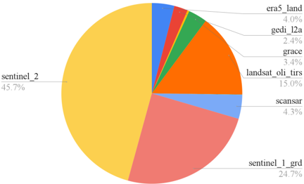
“We find AEF the most performant when trained on the full set of source groups, though with diminishing returns as additional groups are added (Figure 4B).”
§ AlphaEarth Foundations: An embedding field model for accurate and efficient global mapping from sparse label data > Scaling source data quantity and type
plaincorrelational- Asserted: passes — The authors put it forward as true.
- Checkable: passes — It can be checked against evidence.
- Load-bearing: passes — The paper’s conclusions depend on it.
- Based: passes — The paper gives a reason why it holds.
It may state two separate claims as one.
A result the paper reports from its own data — it cites no other source for it, so there is none to check. The quote shows it is in the paper.
In the paper
“In the maxtrial setting with unsupervised thresholding, AEF exceeds performance of all other baselines when detecting land cover change (Figure 3), but not land use change, achieving 71.3% ± 1.14 BA and 71.4% ± 2.08 BA compared to 67.0% ± 1.28 BA (ViT) and 72.9% ± 1.97 BA (ViT) respectively”
§ AlphaEarth Foundations: An embedding field model for accurate and efficient global mapping from sparse label data > Change detection
plain- Asserted: passes — The authors put it forward as true.
- Checkable: passes — It can be checked against evidence.
- Load-bearing: passes — The paper’s conclusions depend on it.
- Based: passes — The paper gives a reason why it holds.
It may state two separate claims as one.
A result the paper reports from its own data — it cites no other source for it, so there is none to check. The quote shows it is in the paper.
In the paper
“For 500-fold 10-shot trials, AEF error reductions were only > 1.0x in the ~90% confidence interval for 8/15 evaluations with an average range of variation ±0.38x”
§ AlphaEarth Foundations: An embedding field model for accurate and efficient global mapping from sparse label data > S6.1. Comparisons with 10 and 1 samples perclass
plain- Asserted: passes — The authors put it forward as true.
- Checkable: passes — It can be checked against evidence.
- Load-bearing: passes — The paper’s conclusions depend on it.
- Based: passes — The paper gives a reason why it holds.
It may state two separate claims as one.
A result the paper reports from its own data — it cites no other source for it, so there is none to check. The quote shows it is in the paper.
In the paper
“While tuning was not performed, as expected, evaluation scores improved when batch uniformity was present, or there was no difference.”
§ AlphaEarth Foundations: An embedding field model for accurate and efficient global mapping from sparse label data > S2.2.4. Batch uniformity objective
plain- Asserted: passes — The authors put it forward as true.
- Checkable: passes — It can be checked against evidence.
- Load-bearing: unclear — It is unclear whether the paper’s conclusions depend on it.
- Based: passes — The paper gives a reason why it holds.
It may state two separate claims as one.
A result the paper reports from its own data — it cites no other source for it, so there is none to check. The quote shows it is in the paper.
In the paper
“The next-best baseline achieved 72.0% ± 1.28 BA (MOSAIKS, kNN, k=3) and 71.5% ± 2.33 BA (composite, kNN, k=3) respectively.”
§ AlphaEarth Foundations: An embedding field model for accurate and efficient global mapping from sparse label data > Change detection
plain- Asserted: passes — The authors put it forward as true.
- Checkable: passes — It can be checked against evidence.
- Load-bearing: passes — The paper’s conclusions depend on it.
- Based: passes — The paper gives a reason why it holds.
It may state two separate claims as one.
A result the paper reports from its own data — it cites no other source for it, so there is none to check. The quote shows it is in the paper.
In the paper
“In characterizing evapotranspiration, AEF demonstrates a significant departure from the other baselines tested being the only method with 𝑅 2 > 0.2, achieving 𝑅 2 = 0.58 ± 0.01 (Figure 3).”
§ AlphaEarth Foundations: An embedding field model for accurate and efficient global mapping from sparse label data > Estimating biophysical variables
boostedcorrelational- Asserted: passes — The authors put it forward as true.
- Checkable: passes — It can be checked against evidence.
- Load-bearing: passes — The paper’s conclusions depend on it.
- Based: passes — The paper gives a reason why it holds.
It may state two separate claims as one.
A result the paper reports from its own data — it cites no other source for it, so there is none to check. The quote shows it is in the paper.
In the paper
“Interestingly, we found that in some cases, controls were selected as the second-best approach, specifically the XYZ control for the Descals oil palm evaluation and the ViT for the LCMAP land use evaluation.”
§ AlphaEarth Foundations: An embedding field model for accurate and efficient global mapping from sparse label data > S6.2. Classification
plain- Asserted: passes — The authors put it forward as true.
- Checkable: passes — It can be checked against evidence.
- Load-bearing: unclear — It is unclear whether the paper’s conclusions depend on it.
- Based: passes — The paper gives a reason why it holds.
It may state two separate claims as one.
A result the paper reports from its own data — it cites no other source for it, so there is none to check. The quote shows it is in the paper.
In the paper
“We found settings of 𝑏 = 0 and 𝑏 = 0.1 to be the least performant across evaluations, and 𝑏 = 0.005 to be optimal.”
§ AlphaEarth Foundations: An embedding field model for accurate and efficient global mapping from sparse label data > S2.2.4. Batch uniformity objective
plain- Asserted: passes — The authors put it forward as true.
- Checkable: passes — It can be checked against evidence.
- Load-bearing: unclear — It is unclear whether the paper’s conclusions depend on it.
- Based: passes — The paper gives a reason why it holds.
It may state two separate claims as one.
A result the paper reports from its own data — it cites no other source for it, so there is none to check. The quote shows it is in the paper.
In the paper
“In the maxtrial setting with unsupervised thresholding, AEF exceeds performance of all other baselines when detecting land cover change (Figure 3), but not land use change, achieving 71.3% ± 1.14 BA and 71.4% ± 2.08 BA compared to 67.0% ± 1.28 BA (ViT) and 72.9% ± 1.97 BA (ViT) respectively”
§ AlphaEarth Foundations: An embedding field model for accurate and efficient global mapping from sparse label data > Change detection
plaincorrelational- Asserted: passes — The authors put it forward as true.
- Checkable: passes — It can be checked against evidence.
- Load-bearing: passes — The paper’s conclusions depend on it.
- Based: passes — The paper gives a reason why it holds.
It may state two separate claims as one.
A result the paper reports from its own data — it cites no other source for it, so there is none to check. The quote shows it is in the paper.
In the paper
“GLanCE land cover max-trial linear transfer BA scores were ~66.6% for 𝑏 = 0.005 and ~64.7% for b = 0.”
§ AlphaEarth Foundations: An embedding field model for accurate and efficient global mapping from sparse label data > S2.2.4. Batch uniformity objective
plain- Asserted: passes — The authors put it forward as true.
- Checkable: passes — It can be checked against evidence.
- Load-bearing: unclear — It is unclear whether the paper’s conclusions depend on it.
- Based: passes — The paper gives a reason why it holds.
It may state two separate claims as one.
The paper states this without a source or data behind it here, so there is nothing to check it against. The quote shows it is in the paper.
In the paper
“resulting in a final total of 15 derivative datasets (Table 1).”
§ AlphaEarth Foundations: An embedding field model for accurate and efficient global mapping from sparse label data > S3.2. Processing
plaindirect- Asserted: passes — The authors put it forward as true.
- Checkable: passes — It can be checked against evidence.
- Load-bearing: fails — The paper’s conclusions may not depend on it.
- Based: passes — The paper gives a reason why it holds.
Probably not a substantial claim. The paper’s conclusions may not depend on it.
A result the paper reports from its own data — it cites no other source for it, so there is none to check. The quote shows it is in the paper.
In the paper
“We found the version described here the most performant, and surprisingly more performant than non-controls in a number of instances.”
§ AlphaEarth Foundations: An embedding field model for accurate and efficient global mapping from sparse label data > S5.1.1. XY
plaincorrelational- Asserted: passes — The authors put it forward as true.
- Checkable: passes — It can be checked against evidence.
- Load-bearing: unclear — It is unclear whether the paper’s conclusions depend on it.
- Based: passes — The paper gives a reason why it holds.
It may state two separate claims as one.
The paper states this without a source or data behind it here, so there is nothing to check it against. The quote shows it is in the paper.
In the paper
“Sat-CLIP was the next-best approach for Ethiopia crops and US trees”
§ AlphaEarth Foundations: An embedding field model for accurate and efficient global mapping from sparse label data > S6.2. Classification
plain- Asserted: passes — The authors put it forward as true.
- Checkable: passes — It can be checked against evidence.
- Load-bearing: unclear — It is unclear whether the paper’s conclusions depend on it.
- Based: passes — The paper gives a reason why it holds.
It may state two separate claims as one.
A result the paper reports from its own data — it cites no other source for it, so there is none to check. The quote shows it is in the paper.
In the paper
“AEF had the highest 𝑅 2 (0.72 ± 0.00), followed by MOSAIKS (0.69 ± 0.00).”
§ AlphaEarth Foundations: An embedding field model for accurate and efficient global mapping from sparse label data > Estimating biophysical variables
plain- Asserted: passes — The authors put it forward as true.
- Checkable: passes — It can be checked against evidence.
- Load-bearing: passes — The paper’s conclusions depend on it.
- Based: passes — The paper gives a reason why it holds.
It may state two separate claims as one.
A result the paper reports from its own data — it cites no other source for it, so there is none to check. The quote shows it is in the paper.
In the paper
“we chose to quantize to 8-bits with power = 2 as this gave the best storage / performance tradeoff based on evaluation performance”
§ AlphaEarth Foundations: An embedding field model for accurate and efficient global mapping from sparse label data > Additional information
plaindirect- Asserted: passes — The authors put it forward as true.
- Checkable: passes — It can be checked against evidence.
- Load-bearing: fails — The paper’s conclusions may not depend on it.
- Based: passes — The paper gives a reason why it holds.
Probably not a substantial claim. The paper’s conclusions may not depend on it.
A result the paper reports from its own data — it cites no other source for it, so there is none to check. The quote shows it is in the paper.
In the paper
“We find generally less differentiation in performance across methods, with the exception of Prithvi and linear trials of MOSAIKS, which perform at or near the random baseline (Figure S19).”
§ AlphaEarth Foundations: An embedding field model for accurate and efficient global mapping from sparse label data > S6.4. Change detection
plain- Asserted: passes — The authors put it forward as true.
- Checkable: passes — It can be checked against evidence.
- Load-bearing: unclear — It is unclear whether the paper’s conclusions depend on it.
- Based: passes — The paper gives a reason why it holds.
It may state two separate claims as one.
The paper states this without a source or data behind it here, so there is nothing to check it against. The quote shows it is in the paper.
In the paper
“We identified and fixed a bug in our processing software that where incorrect handling of time codes for Sentinel-2 images acquired on January 1 resulted in divergent embedding values and visible swath artifacts in affected years.”
§ AlphaEarth Foundations: An embedding field model for accurate and efficient global mapping from sparse label data > S8.3. Production model (AEF v2.1)
plaindirect- Asserted: passes — The authors put it forward as true.
- Checkable: passes — It can be checked against evidence.
- Load-bearing: fails — The paper’s conclusions may not depend on it.
- Based: passes — The paper gives a reason why it holds.
Probably not a substantial claim. The paper’s conclusions may not depend on it.
A result the paper reports from its own data — it cites no other source for it, so there is none to check. The quote shows it is in the paper.
In the paper
“There is some unpredictable nonmonotonicity for some evals, but we do not identify any obvious grouping or regional bias.”
§ AlphaEarth Foundations: An embedding field model for accurate and efficient global mapping from sparse label data > S7.1. Training observations
plain- Asserted: passes — The authors put it forward as true.
- Checkable: passes — It can be checked against evidence.
- Load-bearing: unclear — It is unclear whether the paper’s conclusions depend on it.
- Based: passes — The paper gives a reason why it holds.
It may state two separate claims as one.
A result the paper reports from its own data — it cites no other source for it, so there is none to check. The quote shows it is in the paper.
In the paper
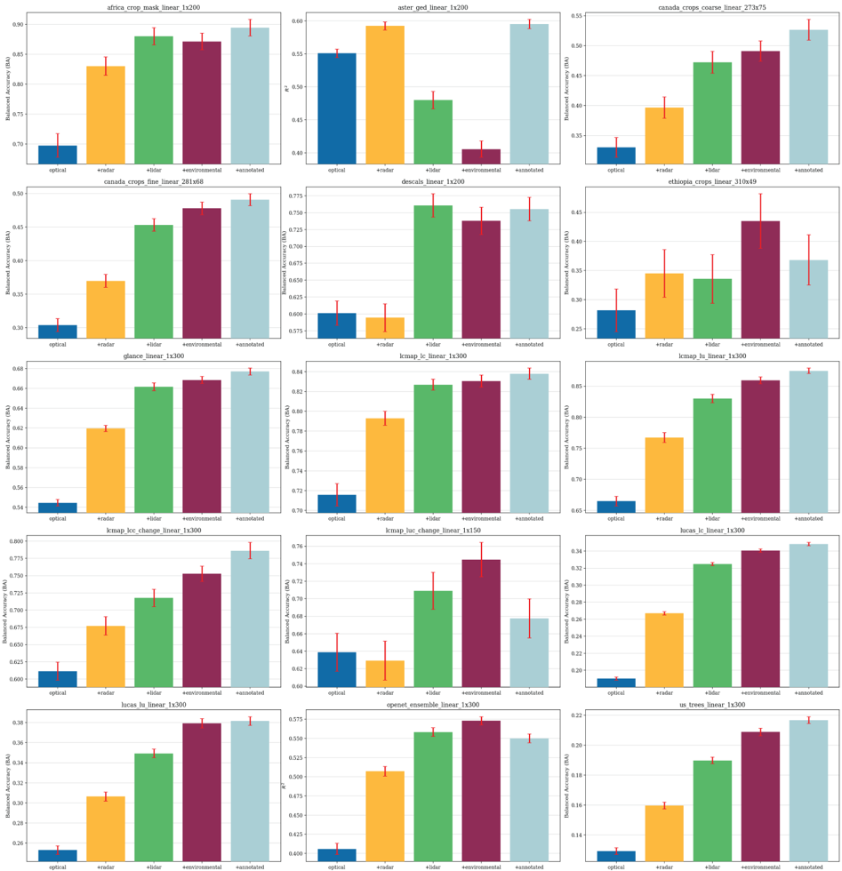
“Unsurprisingly, all LULC evaluations (excluding change) are most performant with all groups including the Annotated group, though interestingly this does not lead to the biggest performance gain compared to adding radar and lidar data.”
§ AlphaEarth Foundations: An embedding field model for accurate and efficient global mapping from sparse label data > S7.2. Sources
plaindirect- Asserted: passes — The authors put it forward as true.
- Checkable: passes — It can be checked against evidence.
- Load-bearing: unclear — It is unclear whether the paper’s conclusions depend on it.
- Based: passes — The paper gives a reason why it holds.
It may state two separate claims as one.
The paper states this without a source or data behind it here, so there is nothing to check it against. The quote shows it is in the paper.
In the paper
“Embeddings generated with AEF v2.1 now use a full year of imagery for inference.”
§ AlphaEarth Foundations: An embedding field model for accurate and efficient global mapping from sparse label data > S8.3. Production model (AEF v2.1)
plain- Asserted: passes — The authors put it forward as true.
- Checkable: passes — It can be checked against evidence.
- Load-bearing: fails — The paper’s conclusions may not depend on it.
- Based: passes — The paper gives a reason why it holds.
Probably not a substantial claim. The paper’s conclusions may not depend on it.
The paper states this without a source or data behind it here, so there is nothing to check it against. The quote shows it is in the paper.
In the paper
“We identified and fixed a bug in our processing software where frame sub-sampling, like that during training, was applied at inference time.”
§ AlphaEarth Foundations: An embedding field model for accurate and efficient global mapping from sparse label data > S8.3. Production model (AEF v2.1)
plain- Asserted: passes — The authors put it forward as true.
- Checkable: passes — It can be checked against evidence.
- Load-bearing: fails — The paper’s conclusions may not depend on it.
- Based: passes — The paper gives a reason why it holds.
Probably not a substantial claim. The paper’s conclusions may not depend on it.
A result the paper reports from its own data — it cites no other source for it, so there is none to check. The quote shows it is in the paper.
In the paper
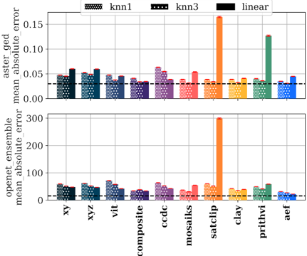
“Here we can more clearly see variability in performance, with particularly large errors for SatCLIP and Prithvi linear trials.”
§ AlphaEarth Foundations: An embedding field model for accurate and efficient global mapping from sparse label data > S6.3. Regression
boostedcorrelational- Asserted: passes — The authors put it forward as true.
- Checkable: passes — It can be checked against evidence.
- Load-bearing: unclear — It is unclear whether the paper’s conclusions depend on it.
- Based: passes — The paper gives a reason why it holds.
It may state two separate claims as one.
A result the paper reports from its own data — it cites no other source for it, so there is none to check. The quote shows it is in the paper.
In the paper
“We find that 𝑅 2 values for AEF are always within a valid range, noting that several other approaches produced negative 𝑅 2 values i.e. worse-than-null performance for ASTER GED (emissivity prediction).”
§ AlphaEarth Foundations: An embedding field model for accurate and efficient global mapping from sparse label data > S6.3. Regression
plain- Asserted: passes — The authors put it forward as true.
- Checkable: passes — It can be checked against evidence.
- Load-bearing: unclear — It is unclear whether the paper’s conclusions depend on it.
- Based: passes — The paper gives a reason why it holds.
It may state two separate claims as one.
The paper states this without a source or data behind it here, so there is nothing to check it against. The quote shows it is in the paper.
In the paper
“Evidently, different evaluations”
§ AlphaEarth Foundations: An embedding field model for accurate and efficient global mapping from sparse label data > S7.2. Sources
plaindirectSingle case- Asserted: passes — The authors put it forward as true.
- Checkable: passes — It can be checked against evidence.
- Load-bearing: unclear — It is unclear whether the paper’s conclusions depend on it.
- Based: passes — The paper gives a reason why it holds.
It may state two separate claims as one.
The paper states this without a source or data behind it here, so there is nothing to check it against. The quote shows it is in the paper.
In the paper
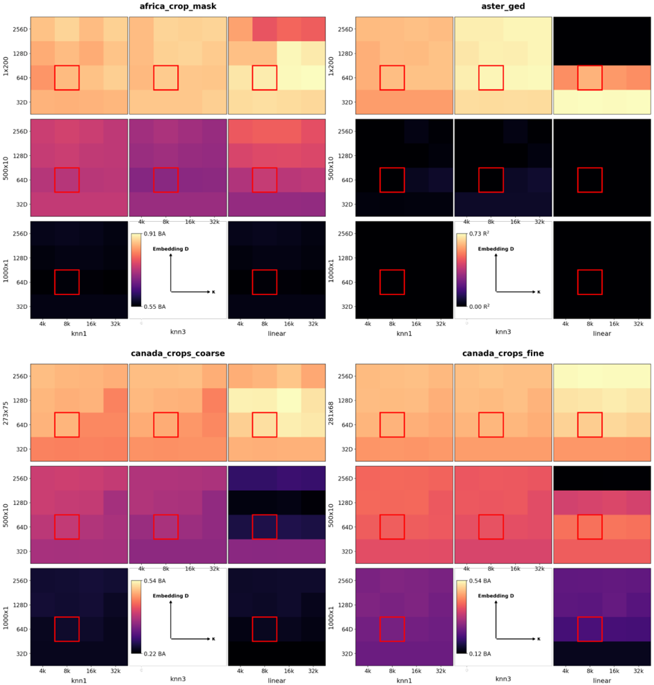
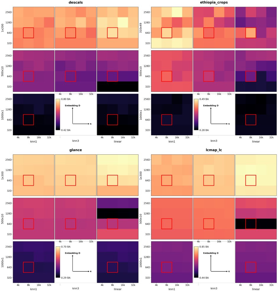
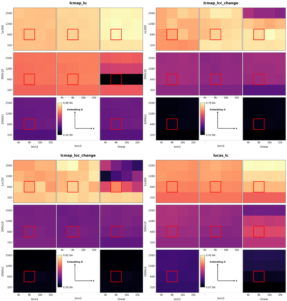
“We also, expectedly, find that a noisier bottleneck seems to improve, or not impact, the performance in the smaller trial groups (500x10, 1000x1).”
§ AlphaEarth Foundations: An embedding field model for accurate and efficient global mapping from sparse label data > S7.3. Bottleneck characteristics
hedgedconditional- Asserted: passes — The authors put it forward as true.
- Checkable: passes — It can be checked against evidence.
- Load-bearing: unclear — It is unclear whether the paper’s conclusions depend on it.
- Based: passes — The paper gives a reason why it holds.
It may state two separate claims as one.
A result the paper reports from its own data — it cites no other source for it, so there is none to check. The quote shows it is in the paper.
In the paper
“We note a variety of patterns characterized by source groups, though 11-of-15 evaluations were most performant with all groups.”
§ AlphaEarth Foundations: An embedding field model for accurate and efficient global mapping from sparse label data > S7.2. Sources
plaincorrelational- Asserted: passes — The authors put it forward as true.
- Checkable: passes — It can be checked against evidence.
- Load-bearing: unclear — It is unclear whether the paper’s conclusions depend on it.
- Based: passes — The paper gives a reason why it holds.
It may state two separate claims as one.
A result the paper reports from its own data — it cites no other source for it, so there is none to check. The quote shows it is in the paper.
In the paper
“For predicting ASTER emissivity values, MO-SAIKS is the next-best approach and composites generally show strong performance, while spectral-temporal CCDC features and XY and XYZ positional encodings are demonstrably worse.”
§ AlphaEarth Foundations: An embedding field model for accurate and efficient global mapping from sparse label data > S6.3. Regression
boostedcorrelational- Asserted: passes — The authors put it forward as true.
- Checkable: passes — It can be checked against evidence.
- Load-bearing: unclear — It is unclear whether the paper’s conclusions depend on it.
- Based: passes — The paper gives a reason why it holds.
It may state two separate claims as one.
A result the paper reports from its own data — it cites no other source for it, so there is none to check. The quote shows it is in the paper.
In the paper
“We note no obvious trend among the baselines, indicating methodologies that perform better on some problems more so than others.”
§ AlphaEarth Foundations: An embedding field model for accurate and efficient global mapping from sparse label data > S7.1. Training observations
hedged- Asserted: passes — The authors put it forward as true.
- Checkable: passes — It can be checked against evidence.
- Load-bearing: fails — The paper’s conclusions may not depend on it.
- Based: passes — The paper gives a reason why it holds.
Probably not a substantial claim. The paper’s conclusions may not depend on it. It may state two separate claims as one.
A result the paper reports from its own data — it cites no other source for it, so there is none to check. The quote shows it is in the paper.
In the paper
“This lead to the addition of a large number of samples from Antarctica that had previously been dropped due to limited coverage, and increased the count of our training video sequences from 8,412,511 to 10,182,450 sequences.”
§ AlphaEarth Foundations: An embedding field model for accurate and efficient global mapping from sparse label data > S8.3. Production model (AEF v2.1)
plaindirect- Asserted: passes — The authors put it forward as true.
- Checkable: passes — It can be checked against evidence.
- Load-bearing: unclear — It is unclear whether the paper’s conclusions depend on it.
- Based: passes — The paper gives a reason why it holds.
It may state two separate claims as one.
A result the paper reports from its own data — it cites no other source for it, so there is none to check. The quote shows it is in the paper.
In the paper
“OpenET ensemble (evapotranspiration prediction) was evidently more challenging where almost all other methods had negative values (clipped to -0.01 for plotting purposes; Figure S17).”
§ AlphaEarth Foundations: An embedding field model for accurate and efficient global mapping from sparse label data > S6.3. Regression
boosted- Asserted: passes — The authors put it forward as true.
- Checkable: passes — It can be checked against evidence.
- Load-bearing: fails — The paper’s conclusions may not depend on it.
- Based: passes — The paper gives a reason why it holds.
Probably not a substantial claim. The paper’s conclusions may not depend on it.
A result the paper reports from its own data — it cites no other source for it, so there is none to check. The quote shows it is in the paper.
In the paper
“we were nonetheless pleased to note little performance variability compared to the non-quantized embeddings as shown in Figure S23A-C”
§ AlphaEarth Foundations: An embedding field model for accurate and efficient global mapping from sparse label data > Additional information
plain- Asserted: passes — The authors put it forward as true.
- Checkable: passes — It can be checked against evidence.
- Load-bearing: unclear — It is unclear whether the paper’s conclusions depend on it.
- Based: passes — The paper gives a reason why it holds.
The quote only partly states this claim.
A conclusion the paper draws from its own results — it cites no other source for it, so there is none to check. The quote shows it is in the paper.
In the paper
“When heuristics are carefully chosen, they can offer an efficient mechanism for geographically extrapolating labels and measurements.”
§ AlphaEarth Foundations: An embedding field model for accurate and efficient global mapping from sparse label data > From sparse labels to maps
plainconditional- Asserted: passes — The authors put it forward as true.
- Checkable: passes — It can be checked against evidence.
- Load-bearing: fails — The paper’s conclusions may not depend on it.
- Based: passes — The paper gives a reason why it holds.
Probably not a substantial claim. The paper’s conclusions may not depend on it.
None of the sources cited for this claim could be matched to a paper in Crossref, so there is nothing to check it against.
In the paper
“Many global mapping efforts focus on individual ecosystems like forests (Hansen et al., 2013), water (Pekel et al., 2016), tidal wetlands (Murray et al., 2022a) or other broad legends, e.g., (Brown et al., 2022;Zanaga et al., 2022).”
§ AlphaEarth Foundations: An embedding field model for accurate and efficient global mapping from sparse label data > From sparse labels to maps
What the sources say
- Not matchedcites Hansen et al., 2013
Couldn’t be matched to a paper in Crossref, so it can’t be checked.
- Not matchedcites Pekel et al., 2016
Couldn’t be matched to a paper in Crossref, so it can’t be checked.
- Not matchedcites Murray et al., 2022a
Couldn’t be matched to a paper in Crossref, so it can’t be checked.
plain- Asserted: passes — The authors put it forward as true.
- Checkable: passes — It can be checked against evidence.
- Load-bearing: fails — The paper’s conclusions may not depend on it.
- Based: passes — The paper gives a reason why it holds.
Probably not a substantial claim. The paper’s conclusions may not depend on it.
- Not matched
A conclusion the paper draws from its own results — it cites no other source for it, so there is none to check. The quote shows it is in the paper.
In the paper
“This simplifies the label collection process, allowing trained interpreters to collect larger volumes at scale at the expense of descriptive power for certain use cases.”
§ AlphaEarth Foundations: An embedding field model for accurate and efficient global mapping from sparse label data > From sparse labels to maps
plaindirect- Asserted: passes — The authors put it forward as true.
- Checkable: passes — It can be checked against evidence.
- Load-bearing: fails — The paper’s conclusions may not depend on it.
- Based: passes — The paper gives a reason why it holds.
Probably not a substantial claim. The paper’s conclusions may not depend on it. It may state two separate claims as one.
What the paper did — it cites no source for this, so there is none to check. The quote shows it is in the paper.
In the paper
“We prioritized reference datasets with human-assigned interpretations or physical measurements over model-generated predictions.”
§ AlphaEarth Foundations: An embedding field model for accurate and efficient global mapping from sparse label data > S3.1. Selection criteria
plain- Asserted: passes — The authors put it forward as true.
- Checkable: passes — It can be checked against evidence.
- Load-bearing: passes — The paper’s conclusions depend on it.
- Based: passes — The paper gives a reason why it holds.
Probably not a substantial claim.
A conclusion the paper draws from its own results — it cites no other source for it, so there is none to check. The quote shows it is in the paper.
In the paper
“The next-best approach varies across evaluation dataset and method, indicating both non-uniform progress and that AEF unlocks progress in historically challenging mapping scenarios.”
§ AlphaEarth Foundations: An embedding field model for accurate and efficient global mapping from sparse label data > Evaluation in realistic data-scarce scenarios
hedgeddirect- Asserted: passes — The authors put it forward as true.
- Checkable: passes — It can be checked against evidence.
- Load-bearing: passes — The paper’s conclusions depend on it.
- Based: passes — The paper gives a reason why it holds.
It may state two separate claims as one.
What the paper did — it cites no source for this, so there is none to check. The quote shows it is in the paper.
In the paper
“For all candidate datasets, we required that the georeference of a given annotation was not tied to a specific observation.”
§ AlphaEarth Foundations: An embedding field model for accurate and efficient global mapping from sparse label data > S3.1. Selection criteria
plain- Asserted: passes — The authors put it forward as true.
- Checkable: passes — It can be checked against evidence.
- Load-bearing: passes — The paper’s conclusions depend on it.
- Based: passes — The paper gives a reason why it holds.
Probably not a substantial claim.
The paper states this without a source or data behind it here, so there is nothing to check it against. The quote shows it is in the paper.
In the paper
“We chose these predictors as they are applicable to low-shot data domains and require minimal parameterization which avoids unduly penalizing any given method due to non-optimal hyperparameters.”
§ AlphaEarth Foundations: An embedding field model for accurate and efficient global mapping from sparse label data > S4.1. Predictors
plaindirect- Asserted: passes — The authors put it forward as true.
- Checkable: passes — It can be checked against evidence.
- Load-bearing: passes — The paper’s conclusions depend on it.
- Based: passes — The paper gives a reason why it holds.
Probably not a substantial claim. It may state two separate claims as one.
In the paper
“These measurements can be used to detect changes in the distribution of water across the planet and estimate terrestrial water storage (Landerer and Swenson, 2012).”
§ AlphaEarth Foundations: An embedding field model for accurate and efficient global mapping from sparse label data > S1.7. GRACE (gravity fields)
What the sources say
- Not matchedcites Landerer and Swenson, 2012
Couldn’t be matched to a paper in Crossref, so it can’t be checked.
plaindirect- Asserted: passes — The authors put it forward as true.
- Checkable: passes — It can be checked against evidence.
- Load-bearing: fails — The paper’s conclusions may not depend on it.
- Based: passes — The paper gives a reason why it holds.
Probably not a substantial claim. The paper’s conclusions may not depend on it. It may state two separate claims as one.
- Not matched
None of the sources cited for this claim could be matched to a paper in Crossref, so there is nothing to check it against.
In the paper
“Median composites are fairly standard for optical imagery and tend to be preferred over mean composites because (a) medians preserve observed data values, and (b) are less sensitive to outliers, particularly clouds and cloud shadows which spectrally lie at very extreme bright and dark values.”
§ AlphaEarth Foundations: An embedding field model for accurate and efficient global mapping from sparse label data > S5.2.1. Composites
What the sources say
- Not matchedcites Francini et al., 2023
Couldn’t be matched to a paper in Crossref, so it can’t be checked.
- Not matchedcites Qiu et al., 2023
Couldn’t be matched to a paper in Crossref, so it can’t be checked.
plaindirect- Asserted: passes — The authors put it forward as true.
- Checkable: passes — It can be checked against evidence.
- Load-bearing: fails — The paper’s conclusions may not depend on it.
- Based: passes — The paper gives a reason why it holds.
Probably not a substantial claim. The paper’s conclusions may not depend on it. It may state two separate claims as one.
- Not matched
A conclusion the paper draws from its own results — it cites no other source for it, so there is none to check. The quote shows it is in the paper.
In the paper
“Preference for SatCLIP here suggests encoding localized EO features was beneficial for these tasks, and improvements for SatCLIP relative to the coordinate and ViT controls indicate that these gains can be attributed to inclusion of EO-specific information content.”
§ AlphaEarth Foundations: An embedding field model for accurate and efficient global mapping from sparse label data > S6.2. Classification
hedgeddirect- Asserted: passes — The authors put it forward as true.
- Checkable: passes — It can be checked against evidence.
- Load-bearing: unclear — It is unclear whether the paper’s conclusions depend on it.
- Based: passes — The paper gives a reason why it holds.
It may state two separate claims as one.
What the paper did — it cites no source for this, so there is none to check. The quote shows it is in the paper.
In the paper
“Where applicable, baselines were provided with identical inputs to AEF and baseline hyperparameters were tuned to maximize performance on our evaluation suite (see supplemental materials S5).”
§ AlphaEarth Foundations: An embedding field model for accurate and efficient global mapping from sparse label data > Evaluation in realistic data-scarce scenarios
hedged- Asserted: passes — The authors put it forward as true.
- Checkable: passes — It can be checked against evidence.
- Load-bearing: passes — The paper’s conclusions depend on it.
- Based: passes — The paper gives a reason why it holds.
Probably not a substantial claim. It may state two separate claims as one.
In the paper
“L-band is a longer wavelength radar signal with greater ability to penetrate through dense vegetation, compared with the C-band frequency measured by Sentinel-1, which tends to be more sensitive to sparse and low biomass vegetation, e.g., (Koyama et al., 2022).”
§ AlphaEarth Foundations: An embedding field model for accurate and efficient global mapping from sparse label data > S1.4. PALSAR-2 (L-band SAR)
What the sources say
- Not matchedcites Koyama et al., 2022
Couldn’t be matched to a paper in Crossref, so it can’t be checked.
plaindirect- Asserted: passes — The authors put it forward as true.
- Checkable: passes — It can be checked against evidence.
- Load-bearing: fails — The paper’s conclusions may not depend on it.
- Based: passes — The paper gives a reason why it holds.
Probably not a substantial claim. The paper’s conclusions may not depend on it. It may state two separate claims as one.
- Not matched
What the paper did — it cites no source for this, so there is none to check. The quote shows it is in the paper.
In the paper
“Additionally we introduce a challenging evaluation suite composed of high-quality reference data that attempts to faithfully replicate realistic mapping scenarios.”
§ AlphaEarth Foundations: An embedding field model for accurate and efficient global mapping from sparse label data > AlphaEarth Foundations
hedged- Asserted: passes — The authors put it forward as true.
- Checkable: passes — It can be checked against evidence.
- Load-bearing: passes — The paper’s conclusions depend on it.
- Based: passes — The paper gives a reason why it holds.
Probably not a substantial claim.
A conclusion the paper draws from its own results — it cites no other source for it, so there is none to check. The quote shows it is in the paper.
In the paper
“By separating information pertinent only to the act of measurement from the mutual information across all sources, we are able to compactly describe Earth's surface properties while maintaining robustness to the noise and sparsity inherent to Earth imaging missions.”
§ AlphaEarth Foundations: An embedding field model for accurate and efficient global mapping from sparse label data > Conclusions
plaindirect- Asserted: passes — The authors put it forward as true.
- Checkable: passes — It can be checked against evidence.
- Load-bearing: passes — The paper’s conclusions depend on it.
- Based: unclear — It is unclear why the paper says it holds.
It may state two separate claims as one.
None of the sources cited for this claim could be matched to a paper in Crossref, so there is nothing to check it against.
In the paper
“LiDAR sensors like GEDI use laser pulses to estimate vegetation profiles, which can in turn be used to map canopy height and vegetation biomass, e.g., (Campbell et al., 2021;Potapov et al., 2021).”
§ AlphaEarth Foundations: An embedding field model for accurate and efficient global mapping from sparse label data > S1.6. GEDI (LiDAR)
What the sources say
- Not matchedcites Campbell et al., 2021
Couldn’t be matched to a paper in Crossref, so it can’t be checked.
- Not matchedcites Potapov et al., 2021
Couldn’t be matched to a paper in Crossref, so it can’t be checked.
plaindirect- Asserted: passes — The authors put it forward as true.
- Checkable: passes — It can be checked against evidence.
- Load-bearing: fails — The paper’s conclusions may not depend on it.
- Based: passes — The paper gives a reason why it holds.
Probably not a substantial claim. The paper’s conclusions may not depend on it. It may state two separate claims as one.
- Not matched
A conclusion the paper draws from its own results — it cites no other source for it, so there is none to check. The quote shows it is in the paper.
In the paper
“Like OpenET, we consider ASTER-GED a proxy task that we can use to evaluate performance in terms of reproducing the results of a more complex modelling workflow for estimating a material property.”
§ AlphaEarth Foundations: An embedding field model for accurate and efficient global mapping from sparse label data > S3.3.10. ASTER Global Emissivity Database (GED)
plain- Asserted: passes — The authors put it forward as true.
- Checkable: passes — It can be checked against evidence.
- Load-bearing: fails — The paper’s conclusions may not depend on it.
- Based: passes — The paper gives a reason why it holds.
Probably not a substantial claim. The paper’s conclusions may not depend on it.
What the paper did — it cites no source for this, so there is none to check. The quote shows it is in the paper.
In the paper
“All data sources were used as targets, only input data sources are required at inference-time to generate embedding fields.”
§ AlphaEarth Foundations: An embedding field model for accurate and efficient global mapping from sparse label data > S1.2. Landsat 8 & 9 (optical, thermal)
plain- Asserted: passes — The authors put it forward as true.
- Checkable: passes — It can be checked against evidence.
- Load-bearing: fails — The paper’s conclusions may not depend on it.
- Based: passes — The paper gives a reason why it holds.
Probably not a substantial claim. The paper’s conclusions may not depend on it.
None of the sources cited for this claim could be matched to a paper in Crossref, so there is nothing to check it against.
In the paper
“We found most if not all datasets in existing geospatial bench-Figure 2 | AlphaEarth Foundations.(A) Block diagram of the overall network architecture used for video analysis.Preprocessing converts raw observation data via normalization using global statistics, and acquisition timestamps are converted to sinusoidal timecodes.Individual source encoders transform inputs to the same latent space”
§ AlphaEarth Foundations: An embedding field model for accurate and efficient global mapping from sparse label data > Evaluation in realistic data-scarce scenarios
What the sources say
- Not matchedcites Bountos et al., 2023
Couldn’t be matched to a paper in Crossref, so it can’t be checked.
- Not matchedcites Lacoste et al., 2023
Couldn’t be matched to a paper in Crossref, so it can’t be checked.
plaindirect- Asserted: passes — The authors put it forward as true.
- Checkable: passes — It can be checked against evidence.
- Load-bearing: passes — The paper’s conclusions depend on it.
- Based: passes — The paper gives a reason why it holds.
It may state two separate claims as one.
- Not matched
None of the sources cited for this claim could be matched to a paper in Crossref, so there is nothing to check it against.
In the paper
“It is generally considered the most accurate, up-to-date radar-derived global DEM, e.g., (Guth and Geoffroy, 2021;Simard et al., 2024).”
§ AlphaEarth Foundations: An embedding field model for accurate and efficient global mapping from sparse label data > S1.8. GLO-30 (topography)
What the sources say
- Not matchedcites Guth and Geoffroy, 2021
Couldn’t be matched to a paper in Crossref, so it can’t be checked.
- Not matchedcites Simard et al., 2024
Couldn’t be matched to a paper in Crossref, so it can’t be checked.
plain- Asserted: passes — The authors put it forward as true.
- Checkable: passes — It can be checked against evidence.
- Load-bearing: fails — The paper’s conclusions may not depend on it.
- Based: passes — The paper gives a reason why it holds.
Probably not a substantial claim. The paper’s conclusions may not depend on it.
- Not matched
What the paper did — it cites no source for this, so there is none to check. The quote shows it is in the paper.
In the paper
“Our global AEF training dataset was developed to provide a representative sample of Earth's terrestrial land surface and near-shore ecosystems, while optimizing for coverage across space, time, and availability of data sources.”
§ AlphaEarth Foundations: An embedding field model for accurate and efficient global mapping from sparse label data > S2.1.1. Training site selection
plain- Asserted: passes — The authors put it forward as true.
- Checkable: passes — It can be checked against evidence.
- Load-bearing: passes — The paper’s conclusions depend on it.
- Based: passes — The paper gives a reason why it holds.
It may state two separate claims as one.
In the paper
“Generating semantic embeddings for any location and time is a stated use case for the Clay model, and classification, regression, and detecting changes over time are suggested use-cases by the authors.”
§ AlphaEarth Foundations: An embedding field model for accurate and efficient global mapping from sparse label data > S5.3.3. Clay
What the sources say
- Not matchedcites Clay, 2024
Couldn’t be matched to a paper in Crossref, so it can’t be checked.
plain- Asserted: passes — The authors put it forward as true.
- Checkable: passes — It can be checked against evidence.
- Load-bearing: fails — The paper’s conclusions may not depend on it.
- Based: passes — The paper gives a reason why it holds.
Probably not a substantial claim. The paper’s conclusions may not depend on it. It may state two separate claims as one.
- Not matched
A conclusion the paper draws from its own results — it cites no other source for it, so there is none to check. The quote shows it is in the paper.
In the paper
“We consider the Africa crop mask reference dataset a good proxy for general agricultural land use in landscapes where there has been notable disagreement among existing mapping efforts.”
§ AlphaEarth Foundations: An embedding field model for accurate and efficient global mapping from sparse label data > S3.3.4. Africa crop mask
plaincorrelational- Asserted: passes — The authors put it forward as true.
- Checkable: passes — It can be checked against evidence.
- Load-bearing: passes — The paper’s conclusions depend on it.
- Based: fails — The paper may give no reason why it holds.
Probably not a substantial claim. The paper may give no reason why it holds.
A conclusion the paper draws from its own results — it cites no other source for it, so there is none to check. The quote shows it is in the paper.
In the paper
“AEF shows previously unachievable performance in low-shot regimes with simple classifiers, unlock-ing use cases that may have previously been untenable given sparse observational records and/or highly detailed taxonomies.”
§ AlphaEarth Foundations: An embedding field model for accurate and efficient global mapping from sparse label data > S6.2. Classification
hedgeddirect- Asserted: passes — The authors put it forward as true.
- Checkable: passes — It can be checked against evidence.
- Load-bearing: passes — The paper’s conclusions depend on it.
- Based: passes — The paper gives a reason why it holds.
It may state two separate claims as one.
In the paper
“The Clay Foundation Model is more akin to a traditional ViT differentiated by the use of input metadata at inference time.”
§ AlphaEarth Foundations: An embedding field model for accurate and efficient global mapping from sparse label data > S5.3.3. Clay
What the sources say
- Not matchedcites Clay, 2024
Couldn’t be matched to a paper in Crossref, so it can’t be checked.
plaincorrelational- Asserted: passes — The authors put it forward as true.
- Checkable: passes — It can be checked against evidence.
- Load-bearing: fails — The paper’s conclusions may not depend on it.
- Based: passes — The paper gives a reason why it holds.
Probably not a substantial claim. The paper’s conclusions may not depend on it.
- Not matched
The paper states this without a source or data behind it here, so there is nothing to check it against. The quote shows it is in the paper.
In the paper
“which have the highest available data quality (terrain corrected, well-calibrated radiometry, intercalibrated across sensors)”
§ AlphaEarth Foundations: An embedding field model for accurate and efficient global mapping from sparse label data > S1.2. Landsat 8 & 9 (optical, thermal)
plain- Asserted: passes — The authors put it forward as true.
- Checkable: passes — It can be checked against evidence.
- Load-bearing: passes — The paper’s conclusions depend on it.
- Based: fails — The paper may give no reason why it holds.
Probably not a substantial claim. The paper may give no reason why it holds. It may state two separate claims as one.
The paper states this without a source or data behind it here, so there is nothing to check it against. The quote shows it is in the paper.
In the paper
“Due to differences in handling of spatial, temporal, and channel dimensions and hard-coded data source requirements, it is not always straightforward to apply them to our benchmark or in a comparable manner.”
§ AlphaEarth Foundations: An embedding field model for accurate and efficient global mapping from sparse label data > S5. Baseline comparisons
hedgeddirect- Asserted: passes — The authors put it forward as true.
- Checkable: passes — It can be checked against evidence.
- Load-bearing: fails — The paper’s conclusions may not depend on it.
- Based: passes — The paper gives a reason why it holds.
Probably not a substantial claim. The paper’s conclusions may not depend on it.
The paper states this without a source or data behind it here, so there is nothing to check it against. The quote shows it is in the paper.
In the paper
“Composites are inherently lower-dimensional and orderless (compared with a stack of images which would be higher-dimensional and preserve the time order of observations), but serve as an important baseline for pure spectral information from minimally transformed de-noised/cloud-free image inputs.”
§ AlphaEarth Foundations: An embedding field model for accurate and efficient global mapping from sparse label data > S5.2.1. Composites
plain- Asserted: passes — The authors put it forward as true.
- Checkable: passes — It can be checked against evidence.
- Load-bearing: fails — The paper’s conclusions may not depend on it.
- Based: passes — The paper gives a reason why it holds.
Probably not a substantial claim. The paper’s conclusions may not depend on it. It may state two separate claims as one.
A conclusion the paper draws from its own results — it cites no other source for it, so there is none to check. The quote shows it is in the paper.
In the paper
“Were we to require that all baseline approaches tested share the same sources, many would be artificially penalized or would not have been usable at all.”
§ AlphaEarth Foundations: An embedding field model for accurate and efficient global mapping from sparse label data > S3.1. Selection criteria
hedgeddirect- Asserted: passes — The authors put it forward as true.
- Checkable: fails — It may be too vague to check against evidence.
- Load-bearing: passes — The paper’s conclusions depend on it.
- Based: passes — The paper gives a reason why it holds.
Probably not a substantial claim. It may be too vague to check against evidence. It may state two separate claims as one.
A conclusion the paper draws from its own results — it cites no other source for it, so there is none to check. The quote shows it is in the paper.
In the paper
“We consider the Descals oil palm reference dataset a useful evaluation of performance for subtle land use and tropical commodity mapping.”
§ AlphaEarth Foundations: An embedding field model for accurate and efficient global mapping from sparse label data > S3.3.8. Descals oil palm
plain- Asserted: passes — The authors put it forward as true.
- Checkable: fails — It may be too vague to check against evidence.
- Load-bearing: fails — The paper’s conclusions may not depend on it.
- Based: passes — The paper gives a reason why it holds.
Probably not a substantial claim. It may be too vague to check against evidence. The paper’s conclusions may not depend on it.
In the paper
“We evaluate only the SatCLIP Vit16-L40 model, which outperforms other versions according to the SatCLIP paper (Klemmer et al., 2025).”
§ AlphaEarth Foundations: An embedding field model for accurate and efficient global mapping from sparse label data > S5.3.1. SatCLIP
What the sources say
- Not matchedcites Klemmer et al., 2025
Couldn’t be matched to a paper in Crossref, so it can’t be checked.
plaindirect- Asserted: passes — The authors put it forward as true.
- Checkable: passes — It can be checked against evidence.
- Load-bearing: fails — The paper’s conclusions may not depend on it.
- Based: passes — The paper gives a reason why it holds.
Probably not a substantial claim. The paper’s conclusions may not depend on it. It may state two separate claims as one.
- Not matched
None of the sources cited for this claim could be matched to a paper in Crossref, so there is nothing to check it against.
In the paper
“SatCLIP is a deep learning-based approach that takes inspiration from CLIP approach (Radford et al., 2021), training location and image encoders via contrastive learning and matching images to their corresponding locations (Klemmer et al., 2025).”
§ AlphaEarth Foundations: An embedding field model for accurate and efficient global mapping from sparse label data > S5.3.1. SatCLIP
What the sources say
- Not matchedcites Radford et al., 2021
Couldn’t be matched to a paper in Crossref, so it can’t be checked.
- Not matchedcites Klemmer et al., 2025
Couldn’t be matched to a paper in Crossref, so it can’t be checked.
plaindirect- Asserted: passes — The authors put it forward as true.
- Checkable: passes — It can be checked against evidence.
- Load-bearing: fails — The paper’s conclusions may not depend on it.
- Based: passes — The paper gives a reason why it holds.
Probably not a substantial claim. The paper’s conclusions may not depend on it. It may state two separate claims as one.
- Not matched
What the paper did — it cites no source for this, so there is none to check. The quote shows it is in the paper.
In the paper
“This helps ensure we are sampling across distinct biogeographic assemblages and ecological habitats with uniform preference regardless of total extent.”
§ AlphaEarth Foundations: An embedding field model for accurate and efficient global mapping from sparse label data > RESOLVE ecoregions
plaindirectn = 846- Asserted: passes — The authors put it forward as true.
- Checkable: passes — It can be checked against evidence.
- Load-bearing: passes — The paper’s conclusions depend on it.
- Based: passes — The paper gives a reason why it holds.
Probably not a substantial claim.
What the paper did — it cites no source for this, so there is none to check. The quote shows it is in the paper.
In the paper
“We assess AEF performance using a set of evaluation datasets we derived from ten publiclyavailable reference datasets representing archetypal classification, regression, and change detection use cases (Table 1).”
§ AlphaEarth Foundations: An embedding field model for accurate and efficient global mapping from sparse label data > S3. Evaluation datasets
plain- Asserted: passes — The authors put it forward as true.
- Checkable: passes — It can be checked against evidence.
- Load-bearing: passes — The paper’s conclusions depend on it.
- Based: passes — The paper gives a reason why it holds.
Probably not a substantial claim.
In the paper
“We chose to use the CCDC approach because it is (a) well-known and widely used for remote sensing applications (see Pasquarella et al. (2022) for a review) and (b) has already been run globally and surfaced as a dataset, making it one of the few existing examples of a model-as-dataset currently available globally in a cloud-computing environment.”
§ AlphaEarth Foundations: An embedding field model for accurate and efficient global mapping from sparse label data > S5.2.2. Continuous Change Detection and Classification (CCDC)
What the sources say
- Not matchedcites Pasquarella et al. (2022)
Couldn’t be matched to a paper in Crossref, so it can’t be checked.
boosteddirect- Asserted: passes — The authors put it forward as true.
- Checkable: passes — It can be checked against evidence.
- Load-bearing: passes — The paper’s conclusions depend on it.
- Based: passes — The paper gives a reason why it holds.
It may state two separate claims as one.
- Not matched
What the paper did — it cites no source for this, so there is none to check. The quote shows it is in the paper.
In the paper
“we also required that labels have a clearly defined “valid period” over which the label could be reasonably applied, i.e., a range or instant (annual, monthly, single-date), and this period must intersect 2017 onward”
§ AlphaEarth Foundations: An embedding field model for accurate and efficient global mapping from sparse label data > S3.1. Selection criteria
plain- Asserted: passes — The authors put it forward as true.
- Checkable: passes — It can be checked against evidence.
- Load-bearing: passes — The paper’s conclusions depend on it.
- Based: passes — The paper gives a reason why it holds.
Probably not a substantial claim.
A conclusion the paper draws from its own results — it cites no other source for it, so there is none to check. The quote shows it is in the paper.
In the paper
“While the mean gain was in AEF's favor for both settings, we consider the extreme degree of variability indicative that adequate general 1-shot or 10-shot performance remains an unsolved research frontier.”
§ AlphaEarth Foundations: An embedding field model for accurate and efficient global mapping from sparse label data > S6.1. Comparisons with 10 and 1 samples perclass
hedged- Asserted: passes — The authors put it forward as true.
- Checkable: passes — It can be checked against evidence.
- Load-bearing: passes — The paper’s conclusions depend on it.
- Based: passes — The paper gives a reason why it holds.
It may state two separate claims as one.
A conclusion the paper draws from its own results — it cites no other source for it, so there is none to check. The quote shows it is in the paper.
In the paper
“and provides a mechanism to parameterize the “smoothness” of a given embedding manifold via the VMF concentration.”
§ AlphaEarth Foundations: An embedding field model for accurate and efficient global mapping from sparse label data > S2.2.1. Simulating a continuous observation record
plaindirect- Asserted: passes — The authors put it forward as true.
- Checkable: passes — It can be checked against evidence.
- Load-bearing: fails — The paper’s conclusions may not depend on it.
- Based: passes — The paper gives a reason why it holds.
Probably not a substantial claim. The paper’s conclusions may not depend on it.
None of the sources cited for this claim could be matched to a paper in Crossref, so there is nothing to check it against.
In the paper
“These machine-generated thematic maps are derived from 30 meter multi-season Landsat imagery and rely on a carefully curated training labels, handengineered spatial, spectral and temporal features, and classic machine learning (i.e., decision trees), as well as rigorous post-processing and accuracy assessment (Wickham et al., 2014(Wickham et al., , 2023)).”
§ AlphaEarth Foundations: An embedding field model for accurate and efficient global mapping from sparse label data > S1.9. NLCD (land cover)
What the sources say
- Not matchedcites Wickham et al., 2014
Couldn’t be matched to a paper in Crossref, so it can’t be checked.
- Not matchedcites Wickham et al., 2023
Couldn’t be matched to a paper in Crossref, so it can’t be checked.
plaindirect- Asserted: passes — The authors put it forward as true.
- Checkable: passes — It can be checked against evidence.
- Load-bearing: fails — The paper’s conclusions may not depend on it.
- Based: passes — The paper gives a reason why it holds.
Probably not a substantial claim. The paper’s conclusions may not depend on it. It may state two separate claims as one.
- Not matched
What the paper did — it cites no source for this, so there is none to check. The quote shows it is in the paper.
In the paper
“All data sources were used as targets, only input data sources are required at inference-time to generate embedding fields.”
§ AlphaEarth Foundations: An embedding field model for accurate and efficient global mapping from sparse label data > S1.2. Landsat 8 & 9 (optical, thermal)
plaindirect- Asserted: passes — The authors put it forward as true.
- Checkable: passes — It can be checked against evidence.
- Load-bearing: passes — The paper’s conclusions depend on it.
- Based: passes — The paper gives a reason why it holds.
Probably not a substantial claim.
The paper states this without a source or data behind it here, so there is nothing to check it against. The quote shows it is in the paper.
In the paper
“While Prithvi authors only explicitly suggest its use with additional deep-learning decoders, it is common to transfer ViT-like architectures via linear decoding as we do here.”
§ AlphaEarth Foundations: An embedding field model for accurate and efficient global mapping from sparse label data > S5.3.2. Prithvi
plain- Asserted: passes — The authors put it forward as true.
- Checkable: passes — It can be checked against evidence.
- Load-bearing: fails — The paper’s conclusions may not depend on it.
- Based: fails — The paper may give no reason why it holds.
Probably not a substantial claim. The paper’s conclusions may not depend on it. The paper may give no reason why it holds. It may state two separate claims as one.
The paper states this without a source or data behind it here, so there is nothing to check it against. The quote shows it is in the paper.
In the paper
“The MOSAIKS approach provides a spatially localized representation of input satellite imagery at a specific time, bearing the same lack-of temporal constraints as composites.”
§ AlphaEarth Foundations: An embedding field model for accurate and efficient global mapping from sparse label data > S5.2.3. MOSAIKS
plain- Asserted: passes — The authors put it forward as true.
- Checkable: passes — It can be checked against evidence.
- Load-bearing: fails — The paper’s conclusions may not depend on it.
- Based: passes — The paper gives a reason why it holds.
Probably not a substantial claim. The paper’s conclusions may not depend on it. It may state two separate claims as one.
What the paper did — it cites no source for this, so there is none to check. The quote shows it is in the paper.
In the paper
“we ensured that we had representation of different temporal aggregations across our final set of evaluations (Table 1).”
§ AlphaEarth Foundations: An embedding field model for accurate and efficient global mapping from sparse label data > S3.1. Selection criteria
plain- Asserted: passes — The authors put it forward as true.
- Checkable: passes — It can be checked against evidence.
- Load-bearing: fails — The paper’s conclusions may not depend on it.
- Based: passes — The paper gives a reason why it holds.
Probably not a substantial claim. The paper’s conclusions may not depend on it.
What the paper did — it cites no source for this, so there is none to check. The quote shows it is in the paper.
In the paper
“We only selected datasets where point coordinate data (longitude, latitude) in decimal degrees was sufficiently precise relative to a nominal 10-meter resolution, i.e., at least four decimal”
§ AlphaEarth Foundations: An embedding field model for accurate and efficient global mapping from sparse label data > S3.1. Selection criteria
plain- Asserted: passes — The authors put it forward as true.
- Checkable: passes — It can be checked against evidence.
- Load-bearing: passes — The paper’s conclusions depend on it.
- Based: passes — The paper gives a reason why it holds.
Probably not a substantial claim.
A conclusion the paper draws from its own results — it cites no other source for it, so there is none to check. The quote shows it is in the paper.
In the paper
“We note that the two baselines with explanatory power in this evaluation, composites and MOSAIKS, are simple transformations from raw satellite data, indicating a gap in applicability of both learned and designed featurization approaches prior to AEF.”
§ AlphaEarth Foundations: An embedding field model for accurate and efficient global mapping from sparse label data > Estimating biophysical variables
hedged- Asserted: passes — The authors put it forward as true.
- Checkable: passes — It can be checked against evidence.
- Load-bearing: passes — The paper’s conclusions depend on it.
- Based: passes — The paper gives a reason why it holds.
It may state two separate claims as one.
What the paper did — it cites no source for this, so there is none to check. The quote shows it is in the paper.
In the paper
“Sample points were allocated to train and test splits such that the training datasets were balanced by class (or regularly spaced bins in the case of regression datasets), with no per-class sample exceeding 300 points and the remainder of the points allocated to an unbalanced test split.”
§ AlphaEarth Foundations: An embedding field model for accurate and efficient global mapping from sparse label data > S3.2. Processing
plain- Asserted: passes — The authors put it forward as true.
- Checkable: passes — It can be checked against evidence.
- Load-bearing: fails — The paper’s conclusions may not depend on it.
- Based: passes — The paper gives a reason why it holds.
Probably not a substantial claim. The paper’s conclusions may not depend on it. It may state two separate claims as one.
What the paper did — it cites no source for this, so there is none to check. The quote shows it is in the paper.
In the paper
“We did not generate any of our own annotations for these evaluations; rather, we identified existing datasets that represented high-quality observation/measurement information and could be used with minimal processing.”
§ AlphaEarth Foundations: An embedding field model for accurate and efficient global mapping from sparse label data > S3.1. Selection criteria
plain- Asserted: passes — The authors put it forward as true.
- Checkable: passes — It can be checked against evidence.
- Load-bearing: fails — The paper’s conclusions may not depend on it.
- Based: passes — The paper gives a reason why it holds.
Probably not a substantial claim. The paper’s conclusions may not depend on it. It may state two separate claims as one.
What the paper did — it cites no source for this, so there is none to check. The quote shows it is in the paper.
In the paper
“Point observations were filtered to guarantee a minimum distance of 1.28 km between sampled points in order to reduce spatial autocorrelation between training and test sites (and this process will be hereafter referred to as “spatial proximity filtering”).”
§ AlphaEarth Foundations: An embedding field model for accurate and efficient global mapping from sparse label data > S3.2. Processing
plaindirect- Asserted: passes — The authors put it forward as true.
- Checkable: passes — It can be checked against evidence.
- Load-bearing: passes — The paper’s conclusions depend on it.
- Based: passes — The paper gives a reason why it holds.
Probably not a substantial claim.
What the paper did — it cites no source for this, so there is none to check. The quote shows it is in the paper.
In the paper
“Data sources were selected to represent a diversity of measurement spaces, resolutions, and temporal refresh rates.”
§ AlphaEarth Foundations: An embedding field model for accurate and efficient global mapping from sparse label data > S1.2. Landsat 8 & 9 (optical, thermal)
plain- Asserted: passes — The authors put it forward as true.
- Checkable: passes — It can be checked against evidence.
- Load-bearing: fails — The paper’s conclusions may not depend on it.
- Based: fails — The paper may give no reason why it holds.
Probably not a substantial claim. The paper’s conclusions may not depend on it. The paper may give no reason why it holds.
What the paper did — it cites no source for this, so there is none to check. The quote shows it is in the paper.
In the paper
“In some cases (like OpenET), we do include “model proxy tasks” that sample model-generated predictions, but these were selected with strong justification, e.g., proxying a computationally intensive ensemble approach.”
§ AlphaEarth Foundations: An embedding field model for accurate and efficient global mapping from sparse label data > S3.1. Selection criteria
plain- Asserted: passes — The authors put it forward as true.
- Checkable: passes — It can be checked against evidence.
- Load-bearing: fails — The paper’s conclusions may not depend on it.
- Based: passes — The paper gives a reason why it holds.
Probably not a substantial claim. The paper’s conclusions may not depend on it.
What the paper did — it cites no source for this, so there is none to check. The quote shows it is in the paper.
In the paper
“while no single source is required for inference, training rows require all input sources to be present so they can be artificially dropped.”
§ AlphaEarth Foundations: An embedding field model for accurate and efficient global mapping from sparse label data > S2.1.3. Training sample
plaindirect- Asserted: passes — The authors put it forward as true.
- Checkable: passes — It can be checked against evidence.
- Load-bearing: passes — The paper’s conclusions depend on it.
- Based: passes — The paper gives a reason why it holds.
Probably not a substantial claim.
What the paper did — it cites no source for this, so there is none to check. The quote shows it is in the paper.
In the paper
“We generally avoided harmonized datasets that combine multiple sets of annotations initially collected with differing protocols/criteria since this makes it more difficult to understand/interpret results/errors.”
§ AlphaEarth Foundations: An embedding field model for accurate and efficient global mapping from sparse label data > S3.1. Selection criteria
plaindirect- Asserted: passes — The authors put it forward as true.
- Checkable: passes — It can be checked against evidence.
- Load-bearing: fails — The paper’s conclusions may not depend on it.
- Based: passes — The paper gives a reason why it holds.
Probably not a substantial claim. The paper’s conclusions may not depend on it.
What the paper did — it cites no source for this, so there is none to check. The quote shows it is in the paper.
In the paper
“We preferred point measurements or annotations over polygons, since reasoning about labels for a specific point rather than over a larger area is more straightforward, and this simplifies sampling of embeddings and other feature vectors for comparisons across approaches.”
§ AlphaEarth Foundations: An embedding field model for accurate and efficient global mapping from sparse label data > S3.1. Selection criteria
plaindirect- Asserted: passes — The authors put it forward as true.
- Checkable: passes — It can be checked against evidence.
- Load-bearing: passes — The paper’s conclusions depend on it.
- Based: passes — The paper gives a reason why it holds.
Probably not a substantial claim. It may state two separate claims as one.
The paper states this without a source or data behind it here, so there is nothing to check it against. The quote shows it is in the paper.
In the paper
“For radar imagery, mean composites tend to be more common as the goal is less-so to avoid outliers and select real data values, and more-so to smooth across many noisy observations varying with slight deviations in acquisition geometry.”
§ AlphaEarth Foundations: An embedding field model for accurate and efficient global mapping from sparse label data > S5.2.1. Composites
plaindirect- Asserted: passes — The authors put it forward as true.
- Checkable: passes — It can be checked against evidence.
- Load-bearing: fails — The paper’s conclusions may not depend on it.
- Based: passes — The paper gives a reason why it holds.
Probably not a substantial claim. The paper’s conclusions may not depend on it.
What the paper did — it cites no source for this, so there is none to check. The quote shows it is in the paper.
In the paper
“we were unable to assess change detection evaluations”
§ AlphaEarth Foundations: An embedding field model for accurate and efficient global mapping from sparse label data > Additional information
plain- Asserted: passes — The authors put it forward as true.
- Checkable: passes — It can be checked against evidence.
- Load-bearing: fails — The paper’s conclusions may not depend on it.
- Based: passes — The paper gives a reason why it holds.
Probably not a substantial claim. The paper’s conclusions may not depend on it.
What the paper did — it cites no source for this, so there is none to check. The quote shows it is in the paper.
In the paper
“We note that XYZ is not time-varying, so we were unable to assess change detection evaluations”
§ AlphaEarth Foundations: An embedding field model for accurate and efficient global mapping from sparse label data > Additional information
plaindirect- Asserted: passes — The authors put it forward as true.
- Checkable: passes — It can be checked against evidence.
- Load-bearing: fails — The paper’s conclusions may not depend on it.
- Based: passes — The paper gives a reason why it holds.
Probably not a substantial claim. The paper’s conclusions may not depend on it. It may state two separate claims as one.
A conclusion the paper draws from its own results — it cites no other source for it, so there is none to check. The quote shows it is in the paper.
In the paper
“confirms that Prithvi is not well-suited for this sort of low-shot classification and requires additional fine-tuning.”
§ AlphaEarth Foundations: An embedding field model for accurate and efficient global mapping from sparse label data > S6.2. Classification
plaindirect- Asserted: passes — The authors put it forward as true.
- Checkable: passes — It can be checked against evidence.
- Load-bearing: unclear — It is unclear whether the paper’s conclusions depend on it.
- Based: passes — The paper gives a reason why it holds.
It may state two separate claims as one.
What the paper did — it cites no source for this, so there is none to check. The quote shows it is in the paper.
In the paper
“have been modified to ensure a minimum spacing of 1.28km between sample points”
§ AlphaEarth Foundations: An embedding field model for accurate and efficient global mapping from sparse label data > S8.3. Production model (AEF v2.1)
plain- Asserted: passes — The authors put it forward as true.
- Checkable: passes — It can be checked against evidence.
- Load-bearing: fails — The paper’s conclusions may not depend on it.
- Based: passes — The paper gives a reason why it holds.
Probably not a substantial claim. The paper’s conclusions may not depend on it.
None of the sources cited for this claim have been checked yet.
In the paper
“Prithvi 4.2M observations”
§ AlphaEarth Foundations: An embedding field model for accurate and efficient global mapping from sparse label data > S8.3. Production model (AEF v2.1)
plain- Asserted: passes — The authors put it forward as true.
- Checkable: passes — It can be checked against evidence.
- Load-bearing: fails — The paper’s conclusions may not depend on it.
- Based: passes — The paper gives a reason why it holds.
Probably not a substantial claim. The paper’s conclusions may not depend on it.
The paper states this without a source or data behind it here, so there is nothing to check it against. The quote shows it is in the paper.
In the paper
“XY is not time-varying”
§ AlphaEarth Foundations: An embedding field model for accurate and efficient global mapping from sparse label data > Additional information
plain- Asserted: passes — The authors put it forward as true.
- Checkable: passes — It can be checked against evidence.
- Load-bearing: passes — The paper’s conclusions depend on it.
- Based: passes — The paper gives a reason why it holds.
Probably not a substantial claim.
None of the sources cited for this claim have been checked yet.
In the paper
“Clay 70M”
§ AlphaEarth Foundations: An embedding field model for accurate and efficient global mapping from sparse label data > S8.3. Production model (AEF v2.1)
plain- Asserted: passes — The authors put it forward as true.
- Checkable: passes — It can be checked against evidence.
- Load-bearing: fails — The paper’s conclusions may not depend on it.
- Based: passes — The paper gives a reason why it holds.
Probably not a substantial claim. The paper’s conclusions may not depend on it.
None of the sources cited for this claim have been checked yet.
In the paper
“SatCLIP uses 100k observations”
§ AlphaEarth Foundations: An embedding field model for accurate and efficient global mapping from sparse label data > S8.3. Production model (AEF v2.1)
plain- Asserted: passes — The authors put it forward as true.
- Checkable: passes — It can be checked against evidence.
- Load-bearing: fails — The paper’s conclusions may not depend on it.
- Based: passes — The paper gives a reason why it holds.
Probably not a substantial claim. The paper’s conclusions may not depend on it.
A conclusion the paper draws from its own results — it cites no other source for it, so there is none to check. The quote shows it is in the paper.
In the paper
“This indicates that local spatial patterns and overall reflectance (as opposed to seasonality in reflectance) are important factors for this use case.”
§ AlphaEarth Foundations: An embedding field model for accurate and efficient global mapping from sparse label data > S6.3. Regression
hedgedcorrelational- Asserted: passes — The authors put it forward as true.
- Checkable: passes — It can be checked against evidence.
- Load-bearing: passes — The paper’s conclusions depend on it.
- Based: passes — The paper gives a reason why it holds.
It may state two separate claims as one.
A conclusion the paper draws from its own results — it cites no other source for it, so there is none to check. The quote shows it is in the paper.
In the paper
“We believe the Ethiopia crops evaluation is particularly challenging given its extreme sparsity and fine scale, and so simple nearest neighbor classification was the best method of transfer for a handful of methods.”
§ AlphaEarth Foundations: An embedding field model for accurate and efficient global mapping from sparse label data > S6.2. Classification
plaindirect- Asserted: passes — The authors put it forward as true.
- Checkable: passes — It can be checked against evidence.
- Load-bearing: unclear — It is unclear whether the paper’s conclusions depend on it.
- Based: passes — The paper gives a reason why it holds.
It may state two separate claims as one.
A conclusion the paper draws from its own results — it cites no other source for it, so there is none to check. The quote shows it is in the paper.
In the paper
“we generally expect poor performance on evaluations where landscapes are dynamic (e.g.agriculture).”
§ AlphaEarth Foundations: An embedding field model for accurate and efficient global mapping from sparse label data > Additional information
hedgedconditional- Asserted: passes — The authors put it forward as true.
- Checkable: passes — It can be checked against evidence.
- Load-bearing: fails — The paper’s conclusions may not depend on it.
- Based: passes — The paper gives a reason why it holds.
Probably not a substantial claim. The paper’s conclusions may not depend on it.
What the paper did — it cites no source for this, so there is none to check. The quote shows it is in the paper.
In the paper
“guarantee balanced sample sizes across classes or bins”
§ AlphaEarth Foundations: An embedding field model for accurate and efficient global mapping from sparse label data > S8.3. Production model (AEF v2.1)
plain- Asserted: passes — The authors put it forward as true.
- Checkable: passes — It can be checked against evidence.
- Load-bearing: passes — The paper’s conclusions depend on it.
- Based: passes — The paper gives a reason why it holds.
Probably not a substantial claim.
A conclusion the paper draws from its own results — it cites no other source for it, so there is none to check. The quote shows it is in the paper.
In the paper
“Given the generally poor performance of all methods on this four class classification problem, there are opportunities to improve performance on this type of dataset.”
§ AlphaEarth Foundations: An embedding field model for accurate and efficient global mapping from sparse label data > S6.2. Classification
plain- Asserted: passes — The authors put it forward as true.
- Checkable: fails — It may be too vague to check against evidence.
- Load-bearing: fails — The paper’s conclusions may not depend on it.
- Based: passes — The paper gives a reason why it holds.
Probably not a substantial claim. It may be too vague to check against evidence. The paper’s conclusions may not depend on it.
The paper states this without a source or data behind it here, so there is nothing to check it against. The quote shows it is in the paper.
In the paper
“As a pre-trained vision model for ImageNet, the ViT is limited in its resolution, bands, and han-”
§ AlphaEarth Foundations: An embedding field model for accurate and efficient global mapping from sparse label data > Additional information
plaindirect- Asserted: passes — The authors put it forward as true.
- Checkable: passes — It can be checked against evidence.
- Load-bearing: fails — The paper’s conclusions may not depend on it.
- Based: fails — The paper may give no reason why it holds.
Probably not a substantial claim. The paper’s conclusions may not depend on it. The paper may give no reason why it holds.
The paper states this without a source or data behind it here, so there is nothing to check it against. The quote shows it is in the paper.
In the paper
“The SatCLIP, XY, and XYZ baselines were omitted from change detection comparisons given these approaches are location-only, i.e., have no time handling or way to differentiate between observations at different times.”
§ AlphaEarth Foundations: An embedding field model for accurate and efficient global mapping from sparse label data > S6.4. Change detection
plaindirect- Asserted: passes — The authors put it forward as true.
- Checkable: passes — It can be checked against evidence.
- Load-bearing: fails — The paper’s conclusions may not depend on it.
- Based: passes — The paper gives a reason why it holds.
Probably not a substantial claim. The paper’s conclusions may not depend on it.
In the paper
“Elevation plays a role in both regulating abiotic conditions and may act as a proxy for other terrain-driven process interactions, e.g., (Hof et al., 2012).”
§ AlphaEarth Foundations: An embedding field model for accurate and efficient global mapping from sparse label data > Additional information
What the sources say
- Not matchedcites Hof et al., 2012
Couldn’t be matched to a paper in Crossref, so it can’t be checked.
hedgedconditional- Asserted: passes — The authors put it forward as true.
- Checkable: passes — It can be checked against evidence.
- Load-bearing: passes — The paper’s conclusions depend on it.
- Based: passes — The paper gives a reason why it holds.
It may state two separate claims as one.
- Not matched
The paper relies on this without support.
Designed Earth observation features are often noisy, sensor-dependent, and highly region- and application-specific.
“However, designed features are often noisy, sensor-dependent, and highly region-and application-specific, compounding the challenges inherent to working with satellite imagery and other planetary-scale datasets.”
The paper relies on this without support.
High-quality maps depend on high-quality labeled data.
“High-quality maps depend on high-quality labeled data, yet when working at global scales, a balance must be struck between measurement precision and spatial coverage.”
The paper relies on this without support.
When working at global scales, a balance must be struck between measurement precision and spatial coverage.
“High-quality maps depend on high-quality labeled data, yet when working at global scales, a balance must be struck between measurement precision and spatial coverage.”
The authors state this as an assumption.
The GLO-30 DEM is valid over the entire period of the training set.
“The GLO-30 DEM is assumed to be valid over the entire period of our training set, though we note with natural and man-made phenomena this is not universally true.”
The authors state this as an assumption.
Geocoded text can provide additional context that will help enrich the learned representations.
“we assume that geocoded text can provide additional context that will help enrich our learned representations.”
The authors state this as an assumption.
Batch element pairs u_i and u'_i are effectively uniform random sample pairs from the training set.
“Assuming a uniform sample from the training set, batch element pairs 𝑢 𝑖 and 𝑢 ′ 𝑖 are effectively uniform random sample pairs from the training set”
The paper relies on this without support.
SAR instruments are water vapor (cloud) penetrating and offer consistent ground measurements in the tropics or other persistently cloud areas.
“Notably SAR instruments are water vapor (cloud) penetrating, and offer consistent ground measurements in the tropics or other persistently cloud areas.”
The paper relies on this without support.
Earth observation data is irregular in space and time, with acquisition campaigns not always global, having acquisition periods unique from other instruments, varying as a function of solar angle, coming on and offline for a number of reasons, and atmospheric conditions at the time an observation is made being unpredictable at local scales.
“Earth observation data is irregular in space and time.Acquisition campaigns are not always global, have acquisition periods unique from other instruments, vary as a function of solar angle, come on and offline for a number of reasons, and atmospheric conditions at the time an observation is made are unpredictable at local scales.”
The authors state this as an assumption.
Land cover represents an instantaneous observation of state.
“We assume land cover represents an instantaneous observation of state”
The authors state this as an assumption.
Land use represents an integrated observation of state (e.g., 'forestry' may include periods of tree cover, clearing, and regrowth).
“We assume land use represents an integrated observation of state (e.g., “forestry” may include periods of tree cover, clearing, and regrowth)”
The authors state this as an assumption.
Non-plantation to plantation transitions are more likely than the reverse.
“We assume that non-plantation to plantation transitions are more likely than the reverse”
The authors state this as an assumption.
The Canada crops datasets are a good proxy for performance on multi-level crop classification at a national scale.
“We assume that these datasets are a good proxy for performance on multi-level crop classification at a national scale”
The authors state this as an assumption.
Surface properties are relatively stable at 100-meter resolution.
“We assume surface properties are relatively stable at 100-meter resolution (though acknowledge this introduces added uncertainty in signal).”
The authors state this as an assumption.
The manifold hypothesis holds.
“assuming the manifold hypothesis (Fefferman et al., 2016).”
Self-check
Percentages, sums and reported differences re-computed from the paper’s own numbers.
Each contradiction between two passages listed here was confirmed by an independent check.
Rated minor: it would not touch a result — a value no result rests on, a p-value that stays on the same side of the significance level, or a conflict that is clerical, resolved elsewhere in the paper, or outside its own findings.
In the paper
§ AlphaEarth Foundations: An embedding field model for accurate and efficient global mapping from sparse label data > Evaluation in realistic data-scarce scenarios
“we developed a set of 15 evaluations sourced from 11 openly available datasets.”
§ AlphaEarth Foundations: An embedding field model for accurate and efficient global mapping from sparse label data > S3. Evaluation datasets
“We assess AEF performance using a set of evaluation datasets we derived from ten publiclyavailable reference datasets representing archetypal classification, regression, and change detection use cases (Table 1).”
Rated minor: it would not touch a result — a value no result rests on, a p-value that stays on the same side of the significance level, or a conflict that is clerical, resolved elsewhere in the paper, or outside its own findings.
In the paper
§ AlphaEarth Foundations: An embedding field model for accurate and efficient global mapping from sparse label data > S7.1. Training observations
“We share a full set of plots detailing the performance scaling of AEF relative to other learned baselines as additional observations are added (Figure S21).”
§ AlphaEarth Foundations: An embedding field model for accurate and efficient global mapping from sparse label data > S8.3. Production model (AEF v2.1)
“Figure: S20 Figure S20 | Figure S20 | Effects of scaling observations for evals in linear probe max-trial regime.”
Rated minor: it would not touch a result — a value no result rests on, a p-value that stays on the same side of the significance level, or a conflict that is clerical, resolved elsewhere in the paper, or outside its own findings.
In the paper
“Our final Ethiopia crops evaluation has a total of 873 training points and 1,657 test points after pre-processing and spatial proximity filtering (Figure S9, Table S14).”
§ AlphaEarth Foundations: An embedding field model for accurate and efficient global mapping from sparse label data > S3.3.6. Ethiopia crops
Reported 1657 · recomputed 1956
Rated minor: it would not touch a result — a value no result rests on, a p-value that stays on the same side of the significance level, or a conflict that is clerical, resolved elsewhere in the paper, or outside its own findings.
In the paper
§ AlphaEarth Foundations: An embedding field model for accurate and efficient global mapping from sparse label data > S5.2.2. Continuous Change Detection and Classification (CCDC)
“The final CCDC feature vector or "embedding" has 56 dimensions (8 coefficients for 7 Landsat bands).”
§ AlphaEarth Foundations: An embedding field model for accurate and efficient global mapping from sparse label data > Additional information
“CCDC Designed Harmonic spectral-temporal features 54 Landsat 8/9 (all bands)”
Rated minor: it would not touch a result — a value no result rests on, a p-value that stays on the same side of the significance level, or a conflict that is clerical, resolved elsewhere in the paper, or outside its own findings.
In the paper
§ AlphaEarth Foundations: An embedding field model for accurate and efficient global mapping from sparse label data > S8.3. Production model (AEF v2.1)
“| (Kerner et al., 2024a,b) | | (4 classes) | Saharan | | | | |”
§ AlphaEarth Foundations: An embedding field model for accurate and efficient global mapping from sparse label data > S3.3.4. Africa crop mask
“The dataset includes pointwise (binary) annotations for cropland versus non-cropland in eight Sub-Saharan African countries”
Rated minor: it would not touch a result — a value no result rests on, a p-value that stays on the same side of the significance level, or a conflict that is clerical, resolved elsewhere in the paper, or outside its own findings.
In the paper
§ AlphaEarth Foundations: An embedding field model for accurate and efficient global mapping from sparse label data > S8.3. Production model (AEF v2.1)
“| et al., 2020; Toth et al., | | (15 classes) | | | | | |”
§ AlphaEarth Foundations: An embedding field model for accurate and efficient global mapping from sparse label data > S3.3.2. LUCAS
“This results in a label dataset with 40 land cover classes (Table S8).”
Rated minor: it would not touch a result — a value no result rests on, a p-value that stays on the same side of the significance level, or a conflict that is clerical, resolved elsewhere in the paper, or outside its own findings.
In the paper
“Our final Ethiopia crops evaluation has a total of 873 training points and 1,657 test points after pre-processing and spatial proximity filtering (Figure S9, Table S14).”
§ AlphaEarth Foundations: An embedding field model for accurate and efficient global mapping from sparse label data > S3.3.6. Ethiopia crops
Reported 873 · recomputed 574
Citations
Cites
The publisher hasn’t deposited this paper’s reference list.
Research works printed but not linked: 39
- Y. Cong, S. Khanna, C. Meng, P. Liu, E. Rozi, Y. He, M. Burke, D. Lobell, and S. Ermon. Satmae: Pre- training transformers for temporal and multi- spectral satellite imagery. Advances in Neural Information Processing Systems, 35:197-211, 2022.
- H. Kerner, C. Nakalembe, A. Yang, I. Zvonkov, R. McWeeny, G. Tseng, and I. Becker-Reshef. How accurate are existing land cover maps for agriculture in sub-saharan africa? Scientific Data, 11(1):486, 2024a.
- K. Klemmer, E. Rolf, C. Robinson, L. Mackey, and M. Rußwurm. Satclip: Global, general-purpose location embeddings with satellite imagery. In Proceedings of the AAAI Conference on Artifi- cial Intelligence, volume 39, pages 4347-4355, 2025.
- R. P. Kornfeld, B. W. Arnold, M. A. Gross, N. T. Dahya, W. M. Klipstein, P. F. Gath, and S. Bet- tadpur. Grace-fo: the gravity recovery and cli- mate experiment follow-on mission. Journal of spacecraft and rockets, 56(3):931-951, 2019.
- C. N. Koyama, M. Shimada, M. Watanabe, and T. Tadono. Alos-2/palsar-2 long-term pantropi- cal observation-a paradigm shift in global for- est monitoring. In EUSAR 2022; 14th European Conference on Synthetic Aperture Radar, pages 1-5. VDE, 2022.
- A. Lacoste, N. Lehmann, P. Rodriguez, E. Sherwin, H. Kerner, B. Lütjens, J. Irvin, D. Dao, H. Alemo- hammad, A. Drouin, et al. Geo-bench: Toward foundation models for earth monitoring. Ad- vances in Neural Information Processing Systems, 36:51080-51093, 2023.
- F. W. Landerer and S. Swenson. Accuracy of scaled grace terrestrial water storage estimates. Water resources research, 48(4), 2012.
- J.-S. Lee, T. L. Ainsworth, and Y. Wang. A review of polarimetric sar speckle filtering. In 2017 IEEE International Geoscience and Remote Sens- ing Symposium (IGARSS), pages 5303-5306. IEEE, 2017.
- A. J. Lister, H. Andersen, T. Frescino, D. Gatzi- olis, S. Healey, L. S. Heath, G. C. Liknes, R. McRoberts, G. G. Moisen, M. Nelson, et al. Use of remote sensing data to improve the ef- ficiency of national forest inventories: a case study from the united states national forest in- ventory. Forests, 11(12):1364, 2020.
- M. B. Lyons, N. J. Murray, E. V. Kennedy, E. M. Kovacs, C. Castro-Sanguino, S. R. Phinn, R. B. Acevedo, A. O. Alvarez, C. Say, P. Tudman, et al. New global area estimates for coral reefs from high-resolution mapping. Cell Reports Sustain- ability, 1(2), 2024.
- F. S. Melton, J. Huntington, R. Grimm, J. Her- ring, M. Hall, D. Rollison, T. Erickson, R. Allen, M. Anderson, J. B. Fisher, et al. Openet: Filling a critical data gap in water management for the western united states. JAWRA Journal of the American Water Resources Association, 58 (6):971-994, 2022.
- J. Muñoz-Sabater, E. Dutra, A. Agustí-Panareda, C. Albergel, G. Arduini, G. Balsamo, S. Bous- setta, M. Choulga, S. Harrigan, H. Hersbach, et al. Era5-land: A state-of-the-art global re- analysis dataset for land applications. Earth system science data, 13(9):4349-4383, 2021.
- N. J. Murray, S. R. Phinn, M. DeWitt, R. Ferrari, R. Johnston, M. B. Lyons, N. Clinton, D. Thau, and R. A. Fuller. The global distribution and trajectory of tidal flats. Nature, 565(7738): 222-225, 2019.
- N. J. Murray, S. P. Phinn, R. A. Fuller, M. DeWitt, R. Ferrari, R. Johnston, N. Clinton, and M. B. Lyons. High-resolution global maps of tidal flat ecosystems from 1984 to 2019. Scientific Data, 9(1):542, 2022a.
- N. J. Murray, T. A. Worthington, P. Bunting, S. Duce, V. Hagger, C. E. Lovelock, R. Lucas, M. I. Saunders, M. Sheaves, M. Spalding, et al. High-resolution mapping of losses and gains of earth's tidal wetlands. Science, 376(6594): 744-749, 2022b.
- R. C. Nagy, J. K. Balch, E. K. Bissell, M. E. Cat- tau, N. F. Glenn, B. S. Halpern, N. Ilangakoon, B. Johnson, M. B. Joseph, S. Marconi, et al. Har- nessing the neon data revolution to advance open environmental science with a diverse and data-capable community. Ecosphere, 12(12): e03833, 2021.
- V. J. Pasquarella, P. Arévalo, K. H. Bratley, E. L. Bullock, N. Gorelick, Z. Yang, and R. E. Kennedy. Demystifying landtrendr and ccdc temporal segmentation. International journal of applied earth observation and geoinformation, 110:102806, 2022.
- V. J. Pasquarella, C. F. Brown, W. Czerwinski, and W. J. Rucklidge. Comprehensive quality assess- ment of optical satellite imagery using weakly supervised video learning. In Proceedings of the IEEE/CVF Conference on Computer Vision and Pattern Recognition, pages 2125-2135, 2023.
- F. Pedregosa, G. Varoquaux, A. Gramfort, V. Michel, B. Thirion, O. Grisel, M. Blondel, P. Prettenhofer, R. Weiss, V. Dubourg, et al. Scikit-learn: Machine learning in python. the Journal of machine Learning research, 12:2825- 2830, 2011.
- J.-F. Pekel, A. Cottam, N. Gorelick, and A. S. Bel- ward. High-resolution mapping of global sur- face water and its long-term changes. Nature, 540(7633):418-422, 2016.
- B. Pengra, S. Stehman, J. Horton, R. Auch, S. Kambly, M. Knuppe, D. Sorenson, C. Ro- bison, and J. Taylor. Lcmap conus reference data product 1984-2021 land cover, land use and change process attributes: Us geologi- cal survey data release.[dataset] https://doi. org/10.5066, 2023.
- P. Potin, B. Rosich, P. Grimont, N. Miranda, I. Shurmer, A. O'Connell, R. Torres, and M. Krassenburg. Sentinel-1 mission status. In Proceedings of EUSAR 2016: 11th European Con- ference on Synthetic Aperture Radar, pages 1-6.
- A. Radford, J. W. Kim, C. Hallacy, A. Ramesh, G. Goh, S. Agarwal, G. Sastry, A. Askell, P. Mishkin, J. Clark, et al. Learning transferable visual models from natural language supervi- sion. In International conference on machine learning, pages 8748-8763. PmLR, 2021.
- E. Rolf, J. Proctor, T. Carleton, I. Bolliger, V. Shankar, M. Ishihara, B. Recht, and S. Hsiang. A generalizable and accessible approach to ma- chine learning with global satellite imagery. Na- ture Communications, 12(1):4392, 2021.
- M. Schmitt, S. A. Ahmadi, Y. Xu, G. Taşkin, U. Verma, F. Sica, and R. Hänsch. There are no data like more data: Datasets for deep learn- ing in earth observation. IEEE Geoscience and Remote Sensing Magazine, 11(3):63-97, 2023.
- M. Simard, M. Denbina, C. Marshak, and M. Neu- mann. A global evaluation of radar-derived digital elevation models: Srtm, nasadem, and glo-30. Journal of Geophysical Research: Biogeo- sciences, 129(11):e2023JG007672, 2024.
- R. Stanimirova, K. Tarrio, K. Turlej, K. McAvoy, S. Stonebrook, K.-T. Hu, P. Arévalo, E. L. Bul- lock, Y. Zhang, C. E. Woodcock, et al. A global land cover training dataset from 1984 to 2020. Scientific Data, 10(1):879, 2023.
- X. Sun, B. Wang, Z. Wang, H. Li, H. Li, and K. Fu. Research progress on few-shot learning for remote sensing image interpretation. IEEE Journal of Selected Topics in Applied Earth Ob- servations and Remote Sensing, 14:2387-2402, 2021.
- B. D. Tapley. Gravity model determination from the grace mission. The Journal of the Astronau- tical Sciences, 56(3):273-285, 2008.
- R. Torres, P. Snoeij, D. Geudtner, D. Bibby, M. Davidson, E. Attema, P. Potin, B. Rommen, N. Floury, M. Brown, et al. Gmes sentinel-1 J. Verbesselt, R. Hyndman, G. Newnham, and D. Culvenor. Detecting trend and seasonal changes in satellite image time series. Remote sensing of Environment, 114(1):106-115, 2010.
- J. M. Volk, J. L. Huntington, F. S. Melton, R. Allen, M. Anderson, J. B. Fisher, A. Kilic, A. Ruhoff, G. B. Senay, B. Minor, et al. Assessing the accu- racy of openet satellite-based evapotranspira- tion data to support water resource and land management applications. Nature Water, 2(2): 193-205, 2024.
- J. Wang, K. Sun, T. Cheng, B. Jiang, C. Deng, Y. Zhao, D. Liu, Y. Mu, M. Tan, X. Wang, et al. Deep high-resolution representation learning for visual recognition. IEEE transactions on pattern analysis and machine intelligence, 43 (10):3349-3364, 2020.
- J. C. White, M. Wulder, G. Hobart, J. Luther, T. Hermosilla, P. Griffiths, N. Coops, R. Hall, P. Hostert, A. Dyk, et al. Pixel-based image compositing for large-area dense time series applications and science. Canadian Journal of Remote Sensing, 40(3):192-212, 2014.
- J. Wickham, C. Homer, J. Vogelmann, A. McK- errow, R. Mueller, N. Herold, and J. Coulston. The multi-resolution land characteristics (mrlc) consortium-20 years of development and inte- gration of usa national land cover data. Remote Sensing, 6(8):7424-7441, 2014.
- J. Wickham, S. V. Stehman, D. G. Sorenson, L. Gass, and J. A. Dewitz. Thematic accuracy assessment of the nlcd 2019 land cover for the conterminous united states. GIScience & remote sensing, 60(1):2181143, 2023.
- B. T. Wilson, J. F. Knight, and R. E. McRoberts. Harmonic regression of landsat time series for modeling attributes from national forest inven- tory data. ISPRS journal of Photogrammetry and Remote Sensing, 137:29-46, 2018.
- M. A. Wulder, T. Hermosilla, J. C. White, C. W. Bater, G. Hobart, and S. C. Bronson. De- velopment and implementation of a stand- level satellite-based forest inventory for canada. Forestry: An International Journal of Forest Re- search, 97(4):546-563, 2024.
- Y. Zeng, D. Hao, A. Huete, B. Dechant, J. Berry, J. M. Chen, J. Joiner, C. Frankenberg, B. Bond- Lamberty, Y. Ryu, et al. Optical vegetation indices for monitoring terrestrial ecosystems globally. Nature Reviews Earth & Environment, 3(7):477-493, 2022.
- X. X. Zhu, D. Tuia, L. Mou, G.-S. Xia, L. Zhang, F. Xu, and F. Fraundorfer. Deep learning in remote sensing: A comprehensive review and list of resources. IEEE geoscience and remote sensing magazine, 5(4):8-36, 2017.
Cited by
Sorted by citations
Items 201–300 of 344
Survey Protocol Cards for Crop Maps
Zaytar, A., Tadesse, G. A., Robinson, C., Nair, S. S., Blasch, G., Degerickx, J., Subakanya, M., Bayas, J. C. L., Hacheme, G., Becker‐Reshef, I., et al. (2026) · IEEE Geoscience and Remote Sensing Letters · doi:10.1109/lgrs.2026.3708987
Nakata, N., Liu, J., Chen, G., Nakata, R., & Varadharajan, C. (2026) · Research Square · doi:10.21203/rs.3.rs-9918364/v1
Aalaila, Y., Elhamdi, M., Großmann, G., Jenson, D., Semenova, E., & Vollmer, S. (2026) · arXiv (Cornell University) · doi:10.48550/arxiv.2607.01082
Ramalason, F. N. (2026) · ORBi (University of Liège)
Utilising embeddings for maps of winter wheat and crop rotation in Henan China during 2018-2024
Du, Z., Rao, K., Wu, C., Wang, K., Dong, S., & Wu, Z. (2026) · ISPRS annals of the photogrammetry, remote sensing and spatial information sciences · doi:10.5194/isprs-annals-xi-2-2026-865-2026
Jing, K., Zhang, M., Wu, B., Xie, Y. D., Li, M., Ma, H. F., & Li, Y. (2026) · Big Earth Data · doi:10.1080/20964471.2026.2691477
Qi, W., Yu, L., Liu, T., Wang, Y., Zhou, X., Zhang, Y., Li, X., Zhao, Q., Wu, H., Zheng, S., et al. (2026) · Journal of Remote Sensing · doi:10.34133/remotesensing.1069
Liliana, & Gonçalves, J. (2026) · Research Square · doi:10.21203/rs.3.rs-10285823/v1
Karwowska, K., Sekrecka, A., Slesinski, J., & Lewinska, M. (2026) · ISPRS annals of the photogrammetry, remote sensing and spatial information sciences · doi:10.5194/isprs-annals-xi-3-2026-555-2026
Li, Z., Xiao, J., Tian, F., & Chai, F. (2026) · Journal of Hydrology · doi:10.1016/j.jhydrol.2026.136000
Scalable and Trustworthy Earth Observation Foundation ModelsPreprint
Imtiaz, S. U., Azadani, M. N., & Alamdari, N. (2026) · arXiv (Cornell University) · doi:10.48550/arxiv.2607.07758
Building Capacity in Satellite-Based Earth Observation and HQP Training: Canada as a Use Case
Elshorbagy, A. M. A., Mitchell, S., & Millard, K. (2026) · ISPRS annals of the photogrammetry, remote sensing and spatial information sciences · doi:10.5194/isprs-annals-xi-5-2026-3-2026
Liu, W., Shu, Q., Zhang, H., Zhang, B., He, T., Wen, X., Wang, Y., Wei, R., Rao, X., & Liu, J. (2026) · Remote Sensing · doi:10.3390/rs18142348
Cross-scale species diversity estimation of tropical forest by integrating UAV and satellite data
Zhao, P., Zheng, Z., Xu, C., Ren, L., Wu, J., Deng, Y., Lin, L., Li, J., Zhao, D., & Zeng, Y. (2026) · Ecological Informatics · doi:10.1016/j.ecoinf.2026.103931
Khan, T. (2026) · arXiv (Cornell University) · doi:10.48550/arxiv.2607.10231
Lamahewage, S. H. G., & Witharana, C. (2026) · SSRN Electronic Journal · doi:10.2139/ssrn.7120967
Bing, Z., Jin, C., Zhengchao, C., Zuoqi, C., Xiao, C., Wenjie, F., Suju, L., Liu, L., Yu, L., Liu, Q., et al. (2026) · National Remote Sensing Bulletin · doi:10.11834/jrs.20266221
Zhao, W., Zhong, X., Yu, B., Wang, X., Li, X., Lu, X., Du, Y., & Zhang, Y. (2026) · GIScience & Remote Sensing · doi:10.1080/15481603.2026.2702254
Kawakami, Y., Cayan, D. R., Liu, D., Ma, K., & Corringham, T. (2026) · arXiv (Cornell University) · doi:10.48550/arxiv.2607.16050
GEM-Forest: A Global satellite EMbedding–based map of forests and tree crops for 2020Preprint
Paluba, D., Marsocci, V., Onačillová, K., Quintana, Y. T. P., & Hastie, A. (2026) · Earth System Science Data Discussions · doi:10.5194/essd-2026-495
Väth, P., Sadbhave, B. L., Dejon, D., Schorcht, G., & Gregorová, M. (2026) · arXiv (Cornell University) · doi:10.48550/arxiv.2607.17661
Now We Know? A Systematic Comparison of TerraMind and THORPreprint
Schindlegger, F., Bounegta, K., Meijling, E. G., Jakubik, J., Salberg, A.-B., Forgaard, T. J. L., Longépé, N., & Marsocci, V. (2026) · arXiv (Cornell University) · doi:10.48550/arxiv.2607.18504
Constructing nationally comprehensive annual rice paddy maps for Madagascar from 2017 to 2025Preprint
Kwon, R., Ryu, Y., Nicola, G. D., Randriamady, H., Mudele, O. E., Tapera, T., Jo, H., & Golden, C. D. W. (2026) · Earth System Science Data Discussions · doi:10.5194/essd-2026-518
Geographische Migrationsforschung auf Basis von Fernerkundung und Social-Media-Daten
Mast, J. (2026) · elib (German Aerospace Center) · doi:10.25972/opus-45525
Embeddings based Anomaly Detection for Cleaning Global Crop Type Reference DatasetsPreprint
Shah, S. R. A., Tricht, K. V., Butsko, C., Degerickx, J., & Szantoi, Z. (2026) · arXiv (Cornell University) · doi:10.48550/arxiv.2607.23908
Pomarico, D., Costantino, A., Sanchez, G. R., Bellantuono, L., D'Alò, D., Elia, M., Fania, A., Giordano, F., Kheirkhahan, N., Lafortezza, R., et al. (2026) · Research Square · doi:10.21203/rs.3.rs-10380924/v1
Pickstone, B. J., Anderson, K., Rowlands, S., Hicks, J., Graham, T., Howe, R., & Delahay, R. J. (2026) · Ecological Solutions and Evidence · doi:10.1002/2688-8319.70302
Fusion of AlphaEarth Embeddings and Sentinel-1 Time-Series for Conflict-Related Urban Damage Mapping
Slesinski, J., Karwowska, K., & Lewinska, M. (2026) · The international archives of the photogrammetry, remote sensing and spatial information sciences/International archives of the photogrammetry, remote sensing and spatial information sciences · doi:10.5194/isprs-archives-xlix-b3-2026-1331-2026
TerraNova: A Foundation Model for the AnthropocenePreprint
Rodriguez-Pardo, C., & Tavoni, M. (2026) · arXiv (Cornell University) · doi:10.48550/arxiv.2607.29527
Evolution of crop models: Modeling approaches and software development
Kapoor, A., Beegum, S., Fleisher, D. H., Timlin, D., Ray, C., & Reddy, V. R. (2026) · Ecological Modelling · doi:10.1016/j.ecolmodel.2026.111764
USFGeoAI: Applying LLMs and Foundation Models to Assist in Image Retrieval
Gamracy, H., Sodhi, P., Sphicas, G., D’Souza, D., Garg, P., Gottlieb, N., Gupta, S. S., Maslekar, R., Patterson, A., Steaderman, N., et al. (2026) · The international archives of the photogrammetry, remote sensing and spatial information sciences/International archives of the photogrammetry, remote sensing and spatial information sciences · doi:10.5194/isprs-archives-xlix-b4-2026-125-2026
Geo-Embed: Towards Unified Multimodal Embeddings for Urban UnderstandingPreprint
Li, J., Li, Y., Zhou, J., Zhang, F., & Liu, Y. (2026) · arXiv (Cornell University) · doi:10.48550/arxiv.2608.03826
Sialellia, G., Scheibenreif, L., Wegner, J. D., & Konrad Schindler, B. (2026) · arXiv (Cornell University) · doi:10.48550/arxiv.2608.04792
Li, Z., Jia, H., Huang, W., Zhao, K., & Chen, M. (2026) · ACM SIGKDD Conference on Knowledge Discovery and Data Mining (KDD) · doi:10.1145/3770855.3818168
How Usable Are Geospatial Foundation Models? A Systematic Evaluation of 89 ModelsPreprint
Young, R., Gabtraupov, A., Soror, K., & Keshav, S. (2026) · arXiv (Cornell University) · doi:10.48550/arxiv.2608.03804
Ma, H., & Kwan, M. (2026) · 中国科学通报:英文版 · doi:10.1016/j.scib.2026.08.020
Global mapping of stony desert through few-shot similarity with geospatial foundation models
Wang, J., Lu, N., Sun, Y., Li, L., & Wang, J. (2026) · Geoderma · doi:10.1016/j.geoderma.2026.117982
Cao, Y., Su, F., Fu, D., Wu, W., Yan, F., Fan, R., Chen, H., & Huang, X. (2026) · ISPRS Journal of Photogrammetry and Remote Sensing · doi:10.1016/j.isprsjprs.2026.08.002
SAR2Agri: Learning SAR Intensity Representations for Agricultural MonitoringPreprint
Gupta, M. R., & Sobti, A. (2026) · arXiv (Cornell University)
Di, H., Zhao, Y., Tian, J., Du, X., Li, Q., Zhang, Y., Wang, H., & Luo, J. (2026) · doi:10.31223/x50504
Bahrami, H., Homayouni, S., Champagne, C., McNairn, H. E., Daneshfar, B., Chokmani, K., Nteziyaremye, A., & Zannou, A. (2026) · Big Earth Data · doi:10.1080/20964471.2026.2705616
Rozanov, A. P., Renganathan, A., & Kumar, V. (2026) · arXiv (Cornell University) · doi:10.48550/arxiv.2608.14372
Li, P., Chen, P., Wang, J., Yang, Z., 陈天胜, Gong, M., & Cheng, X. (2026) · arXiv (Cornell University) · doi:10.48550/arxiv.2608.16310
Bridging the weather and climate divide with artificial intelligence
Camps‐Valls, G., Carrassi, A., Viríssimo, F. D. M., Debeire, K., Fernández‐Torres, M., Hess, P., Heuer, H., Mankovich, N., Montero, D., Bonet, E. R., et al. (2026) · Nature Communications · doi:10.1038/s41467-026-75787-y
Toward Causal Reasoning in GeoAI : A Three‐Tier Framework for Spatial Decision Support
Niu, Y., Zhang, Z., Yuan, M., Cheng, T., & Li, W. (2026) · Transactions in GIS · doi:10.1111/tgis.70372 · Cited by 1
MoRAX: Mobility-based Representation Augmentation for Geospatial Foundation ModelsPreprint
Wen, Y., Jixuan Cai, 蔡., Zhou, Y., & Kirkley, A. (2026) · arXiv (Cornell University) · doi:10.48550/arxiv.2608.17848
Temporal Sensitivity Analysis of Tessera EmbeddingsPreprint
Guerrero‐Viu, J., López-Cifuentes, A., Pérez-Villar, I., & Pacifici, F. (2026) · arXiv (Cornell University) · doi:10.48550/arxiv.2608.27175
Huidobro, C. O., & Koren, G. (2026) · Geophysical Research Letters · doi:10.1029/2026gl122340
Flynn, T., Rozanov, A., & Mesele, S. A. (2026) · doi:10.31223/x5jn5t
Foundation Models Meet Agriculture: Challenges Beyond PretrainingPreprint
Nedungadi, V., Xiong, X., Rußwurm, M., & Athanasiadis, I. N. (2026) · arXiv (Cornell University) · doi:10.48550/arxiv.2608.30392
Tian, H., Cai, H., & Yang, Y. (2026) · arXiv (Cornell University) · doi:10.48550/arxiv.2608.29553
Koukos, A., Kondylatos, S., Nord‐Larsen, T., Nyborg, L., Tøttrup, C., & Grogan, K. (2026) · arXiv (Cornell University) · doi:10.48550/arxiv.2609.03480
Ma, X., Qu, Y., Wang, H., Chen, M., Yang, C., Zheng, G., Xu, C., & Bi, Y. (2026) · International Journal of Applied Earth Observation and Geoinformation · doi:10.1016/j.jag.2026.105566
GEDI spaceborne lidar for protected areas monitoring
Cotrina-Sánchez, A., Moudrý, V., Laurin, G. V., Coomes, D., Boukhris, I., Hakkenberg, C. R., Rossi, C., Veneros, J., Coronel-Alcalde, M. N., Alvarez, J., et al. (2026) · Environmental Research Letters · doi:10.1088/1748-9326/aea352
Advancing global urban mapping with multimodal robustness and versatile applications
Zhou, Y., & Weng, Q. (2026) · ISPRS Journal of Photogrammetry and Remote Sensing · doi:10.1016/j.isprsjprs.2026.08.042
Moltzen, K., Banerjee, D., Burmester, J., Ehrenberg, A., Köhler, M., Möller, C., Pfeifer, J., Taffa, T. A., Schulz, H. M., Usmanova, A., et al. (2026) · DROPS (Schloss Dagstuhl – Leibniz Center for Informatics) · doi:10.4230/lipics.cosit.2026.20
Applying foundation model embeddings towards urban livability evaluationPreprint
Khot, A., Zhou, W., & Wang, S. (2026) · arXiv (Cornell University) · doi:10.48550/arxiv.2609.09429
From Equations to Geospatial Foundation models. What comes next for forest prediction?Preprint
Boukhris, I., Bouriaud, O., Sanchez, A., Torresani, M., Valentini, R., & Nakhle, F. (2026) · doi:10.31223/x5z80v
Guthrie, J., Oughton, E. J., Wessels, K., Rice, M., & Corley, I. (2026) · arXiv (Cornell University) · doi:10.48550/arxiv.2609.09482
Hendrix, N., Carl, Z., Heitzig, C., Bazemore, A., & Rehkopf, D. H. (2022) · arXiv (Cornell University) · doi:10.48550/arxiv.2609.11689
Multi-annual sub-pixel land cover mapping with TESSERA latent embeddingsPreprint
Schug, F., Klehr, D., Mahler, J., & Frantz, D. (2026) · doi:10.31223/x59j7c · Cited by 1
Sertel, E., İlmak, D., Aksoy, S., & Ustaoğlu, B. (2026) · International Journal of Digital Earth · doi:10.1080/17538947.2026.2732311
Earth-Agent-Pro: Towards Real-World Full-Chain Earth Observation with AgentsPreprint
Lv, Z., Dang, C., Feng, Y., Gong, Y., Wang, X., Ye, J., He, C., & Li, W. (2026) · arXiv (Cornell University) · doi:10.48550/arxiv.2609.12533
Ten rules to increase the usability of earth observation mission datasets
Scheick, J., Barrett, A. P., Fair, Z., Katz, Z. S., López, L. A., Neeley, A., Roberts, C., Smith, B. E., Snow, T., Wegener, R., et al. (2026) · Earth Science Informatics · doi:10.1007/s12145-026-02216-5
Annual geospatial foundation model embeddings for landslide susceptibility assessment in Taiwan
Fang, J., Luo, W., Huang, Q., Li, W., Chen, Y., & Liu, C. (2026) · npj natural hazards. · doi:10.1038/s44304-026-00268-7
Physically Typed and Geometry-Aware Representations for Earth Foundation ModelsPreprint
Ranjan, R. (2026) · arXiv (Cornell University) · doi:10.48550/arxiv.2609.13868
MoveBench: A Benchmark for Global-Scale Wildlife Movement ForecastingPreprint
Kay, J., Bar, S., Aikens, E. O., Becker, M., Cagnacci, F., Cohen, J., Forrest, S. W., Kendall-Bar, J. M., Lucas, M., Overcast, M., et al. (2026) · arXiv (Cornell University) · doi:10.48550/arxiv.2609.15780
Towards foundation models for insurance risk modellingPreprint
Blier-Wong, C. (2026) · arXiv (Cornell University) · doi:10.48550/arxiv.2609.14576
Mandal, N. C., Hoque, O. B., Luong, K., Swarup, S., Rajagopalan, K., Wilson, M., Adiga, A., & Marathe, M. (2026) · International Joint Conference on Artificial Intelligence · doi:10.24963/ijcai.2026/816
Dutrieux, L. P., Sarah, C., Deutscher, J., Griess, V. C., Milenković, M., Hans, P., Antoni, Z., & Beck, P. S. A. (2026) · Joint Research Centre (European Commission) · doi:10.3929/ethz-c-000806998
Developing Reliable Machine Learning Methods for Earth Observation and Landscape Change
Lin, P.-C. (2026) · ResearchWorks at the University of Washington (University of Washington)
Hamunyela, E., Amukwaya, A., & Hipondoka, M. H. T. (2026) · International Journal of Remote Sensing · doi:10.1080/01431161.2026.2732266
Geography as the Organizing Grammar of Geospatial ModelsPreprint
Ranjan, R., & Tamaskar, S. (2026) · arXiv (Cornell University) · doi:10.48550/arxiv.2609.19621
Foundation models in Earth system science: Advances, challenges, and future paths
Su, F., Cao, Y., Li, X., Wang, H., Fan, R., Huang, S., He, W., Chen, Z., Zhang, P., Zhao, L., et al. (2026) · The Innovation Reviews · doi:10.59717/j.tirv.2026.100014
Dinç, P., Sardar, P., & Ayvazyan, M. (2026) · Environmental Research Letters · doi:10.1088/1748-9326/aeaa71
Kerkad, A., & Gouri, R. (2026) · Advances in intelligent systems and computing · doi:10.1007/978-3-032-27214-0_50
High-resolution Nitrogen Dioxide Maps Reveal Exposure Limit Breaches across EuropePreprint
Scheibenreif, L., & Konrad Schindler, B. (2026) · arXiv (Cornell University) · doi:10.48550/arxiv.2609.24634
Bai, Y., Wang, H., Yin, Y., Cheng, S., He, J., Su, Z., Wang, K., & Li, X. (2026) · International Journal of Applied Earth Observation and Geoinformation · doi:10.1016/j.jag.2026.105604
National-scale mapping locates the mismatch between perceived and assessed flood risk in IndiaPreprint
Tripathy, P., Upadhyay, S., Alegbeleye, O. M., Senkardesler, E., Pingali, D., Goddard, E., Thaker, J. J., Leiserowitz, A., & Marlon, J. R. (2026) · doi:10.31223/x5wz38
Ratsakatika, T., Zotta, M. I., Keshav, S., & Lines, E. R. (2026) · arXiv (Cornell University) · doi:10.48550/arxiv.2609.28194
Tahseen, M., Zaidi, J., Tanvir, K., Nur, K. M., Nazera, F., Sezan, M. S. B. K., & Gomes, D. J. (2026) · Advances in computational intelligence and robotics book series · doi:10.4018/979-8-2600-1704-3.ch001
Sohrabi, H., Daryaei, A., Samaei, R. M., Vafaei, S., Miraki, M., Bavaghar, M. P., Panahi, P., Rajaei, R., Ghorbanzadeh, O., den Dool, G. V., et al. (2026) · doi:10.31223/x5cv4z
Recoverable Geographic Location Information in Earth-Observation EmbeddingsPreprint
Zhang, P., Hu, K., Knežević, J., Yin, S., & Gao, K. (2026) · arXiv (Cornell University) · doi:10.48550/arxiv.2609.29151
dos Anjos, A. E., Ferreira, K. R., & de Queiroz, G. R. (2026) · Biblioteca Digital da Memória Científica do INPE (National Institute for Space Research) · doi:10.5281/zenodo.22981706
On the Value of Images to Learn Ecology-Aware Geographic Embeddings
Menoud, A., Servajean, M., Pavez, P. U., Larcher, T., & Marcos, D. (2026) · Lecture notes in computer science · doi:10.1007/978-3-032-39518-4_27
AlphaEarth distinguishes cities but compresses urban variationPreprint
Renninger, A. (2026) · arXiv (Cornell University) · doi:10.48550/arxiv.2609.30356
Qi, G., Wei, J., Xin, Z., Yao, L., Yuan, H., Nie, M., Li, B., Chen, X., & Ma, J. (2026) · Earth System Science Data Discussions · doi:10.5194/essd-2026-719
Idrees, A., Cabral, P., & Jamal, S. A. (2026) · Soil Use and Management · doi:10.1111/sum.70310
Ganguly, K., & Mitran, T. (2026) · SSRN Electronic Journal · doi:10.2139/ssrn.7525209
When local gains fail to transfer: Frozen Earth-observation embeddings across wildfiresPreprint
Stark, P., Sopasakis, A., & Hall, O. (2026) · arXiv (Cornell University) · doi:10.48550/arxiv.2609.34602
Distributed Hydrological Modeling in the Feature SpacePreprint
Eddin, M. H. S., Taccari, M. L., Zhang, Y., Jiang, S., Gall, J., & Reichstein, M. (2026) · arXiv (Cornell University) · doi:10.48550/arxiv.2609.32971
Nelson, D. R., Plouviez, M., Daakour, S., Jaiswal, A. K., Fu, W., Amin, S. A., & Salehi‐Ashtiani, K. (2026) · SSRN Electronic Journal · doi:10.64898/2026.09.23.753693
Parameter Efficient Handling of Acquisition Artefacts
Tresson, P., Mounziegou‐Mounziegou, C., Marcos, D., Tulet, H., Viennois, G., & Barbier, N. (2026) · Lecture notes in computer science · doi:10.1007/978-3-032-39385-2_40
Planetary Feature Fields are Scalable Earth RepresentationsPreprint
Rao, A., Loeschcke, S., Fuller, A., Corley, I., Lang, N., & Shelhamer, E. (2026) · arXiv (Cornell University) · doi:10.48550/arxiv.2609.37784
Self-citation
Metadata
- Authors
- Brown, C. F., Kazmierski, M. R., Pasquarella, V. J., Rucklidge, W. J., Samsikova, M., Zhang, C., Shelhamer, E., Lahera, E., Wiles, O., Ilyushchenko, S., Gorelick, N., Zhang, L. L., Alj, S., Schechter, E., Askay, S., Guinan, O., Moore, R., Boukouvalas, A., & Kohli, P.
- Venue
- arXiv
- Publisher
- arXiv
- Published
- 2025
- ISSN
- 2331-8422 (ISSN-L)
- arXiv
- 2507.22291
- OpenAlex
- W6948349386
- Semantic Scholar
- 0edf512a0375908943b80777e8abb290354848b2
- Cited by
- 172
- References
- 0
- Citations by year
- 2026: 156 · 2025: 16
- Type
- posted content
- Language
- en
- Open access
- green
- arxiv.org
- Licence
- Locations
- arXiv (Cornell University) (submittedVersion, cc-by-nc)
- arXiv (Cornell University) (cc-by)
- Topics
- Physical Sciences › Computer Science › Computer Vision and Pattern Recognition › Remote-Sensing Image Classification
- Social Sciences › Geography, Planning and Development › Geographic Information Systems Studies
- Life Sciences › Agricultural and Biological Sciences › Soil Science › Soil Geostatistics and Mapping
- Keywords
- global mapping, Earth observation, AlphaEarth Foundations
About these checks
Registry, retraction, Cites and statistics results are computed, not judged, with one exception: a printed reference that no index lists is read once by a model before it counts as a citation error. Claims are extracted by a model and kept only when their quote appears verbatim in the text; each cited source is then checked, with a model’s help, for whether it says what the claim relies on. Those verdicts can be wrong — read the claim’s quote and the cited source before relying on one.
A language model drew the claims from the paper on 2026-11-10, under version 3 of the claim definition (model deepseek-v4.1-flash, prompt extract-v3).
A second model labelled each claim on 2026-11-10 (model jev-1.13-20260917, definition revision gold-guideline-v0.2).
Statistics and arithmetic are recomputed, not judged.
Confidence bands are shown only for fields calibrated on our annotated test set. None is calibrated yet, so no band is shown.
What counts as a claim ›How we measure confidence ›How we check this ›
Are you an author, or do you see a problem with this page? Request a review
