

The DOI matches its Crossref record; 3 of the 3 references it cites were found in a registry or an index.
A distributed hybrid physics–AI framework for learning corrections of internal hydrological fluxes and enhancing high-resolution regionalized flood modeling
Open accessPublished version of a preprint
Abstract
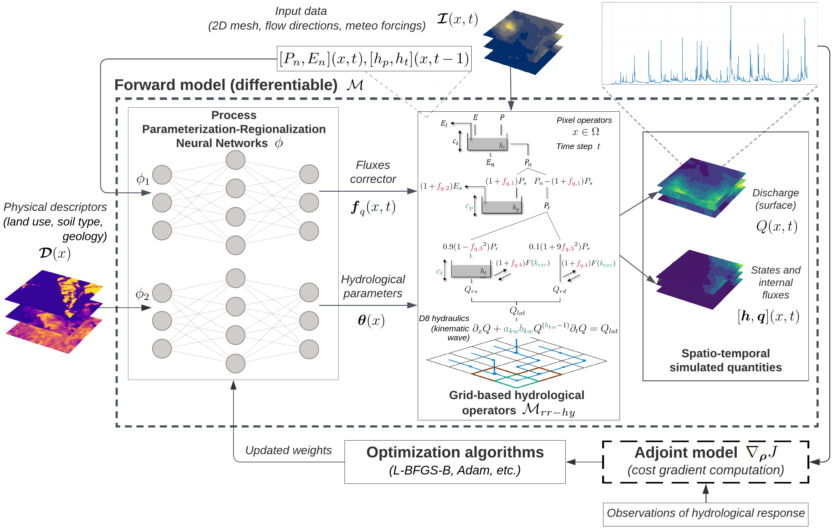
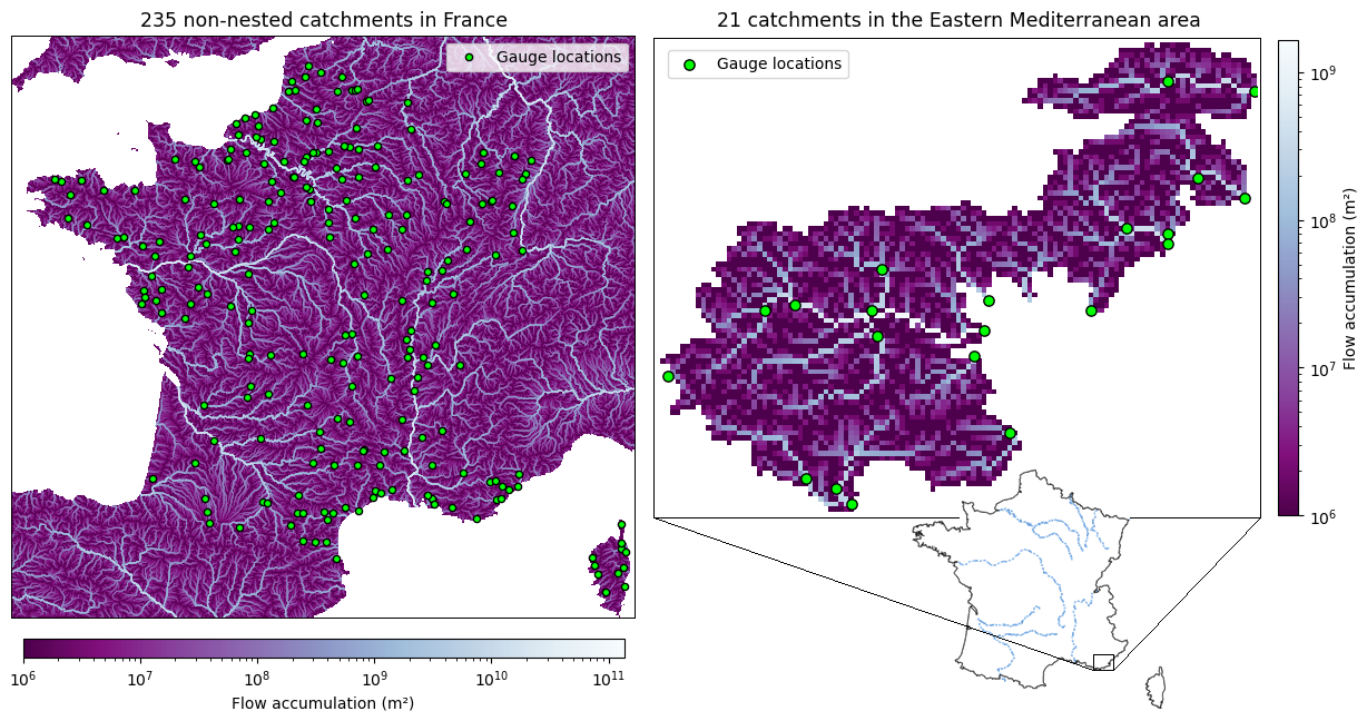
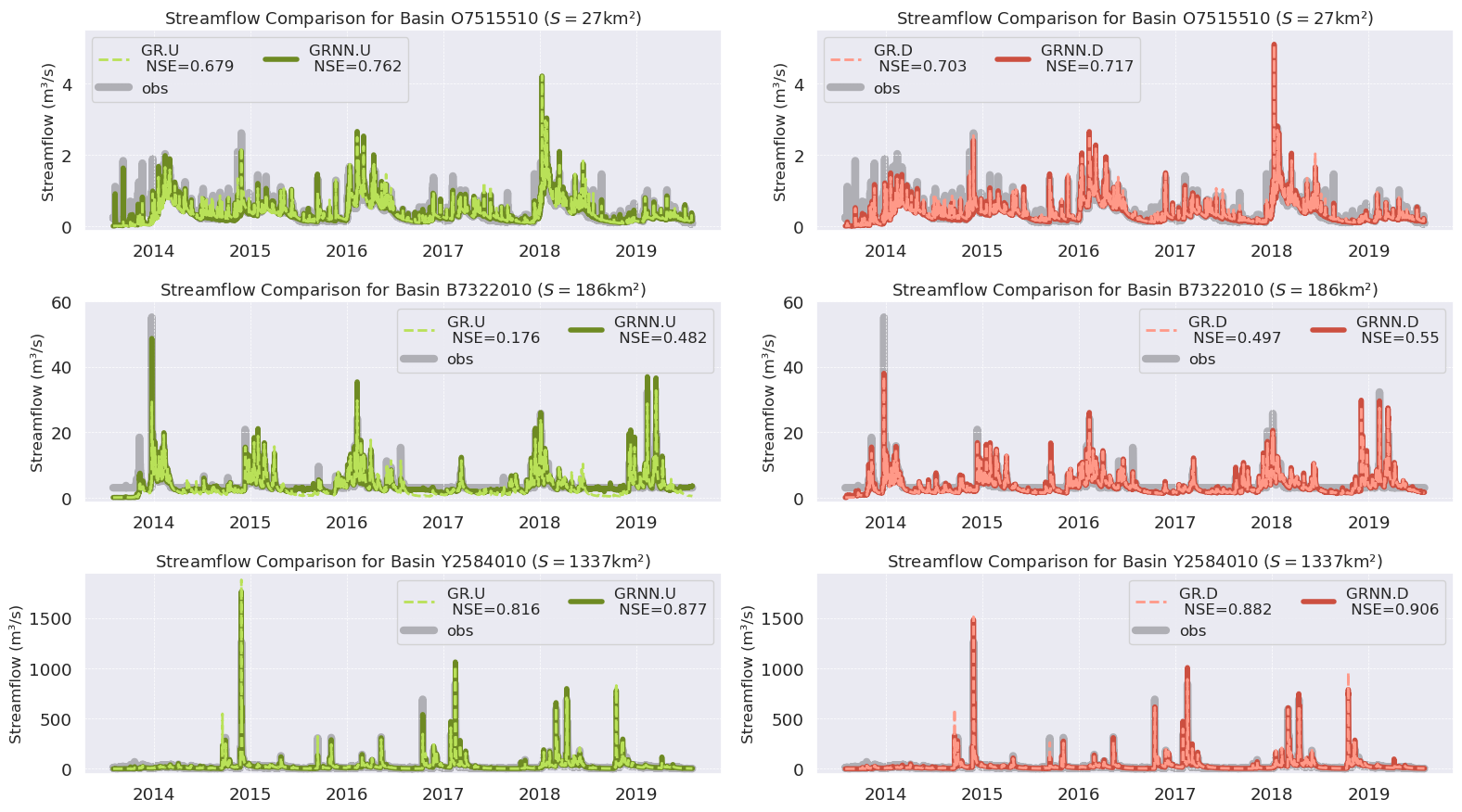
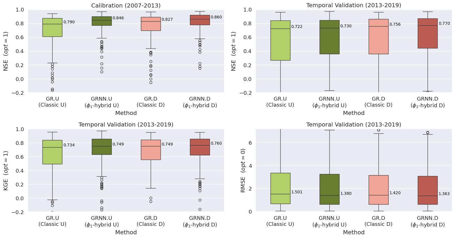
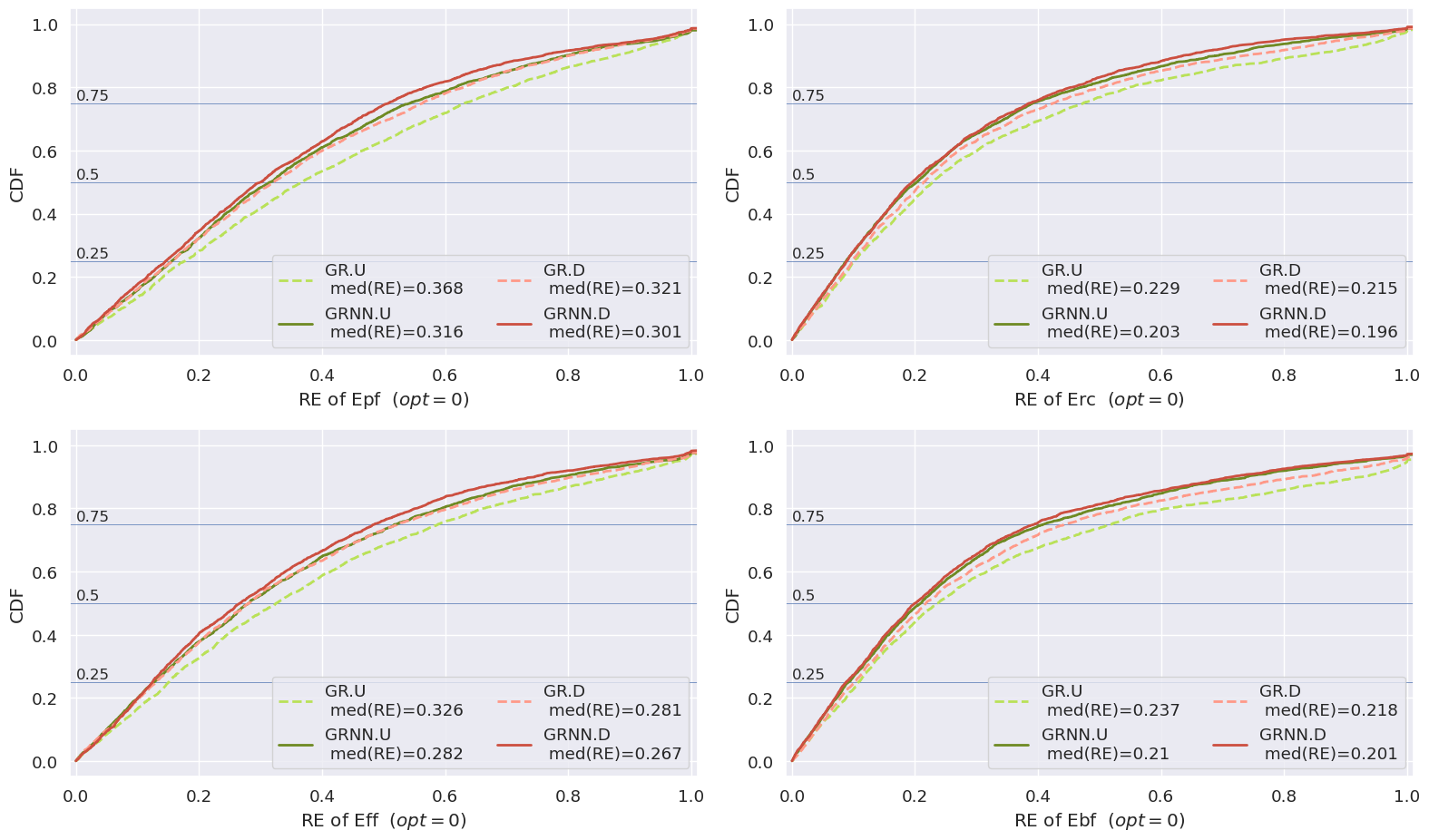
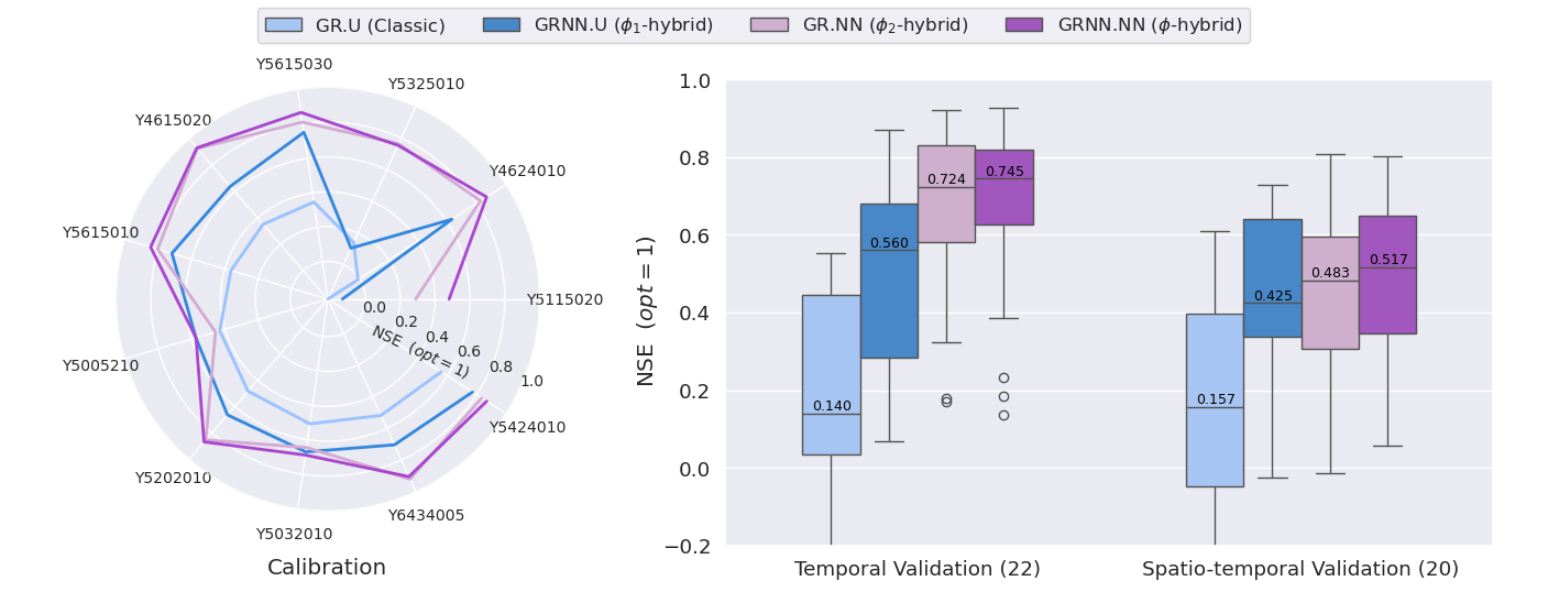
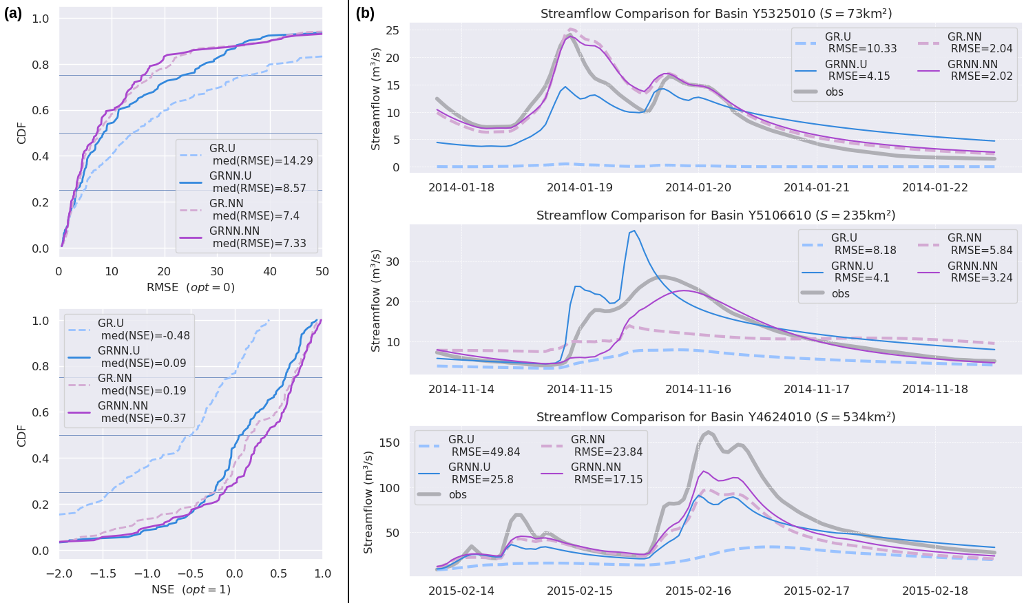
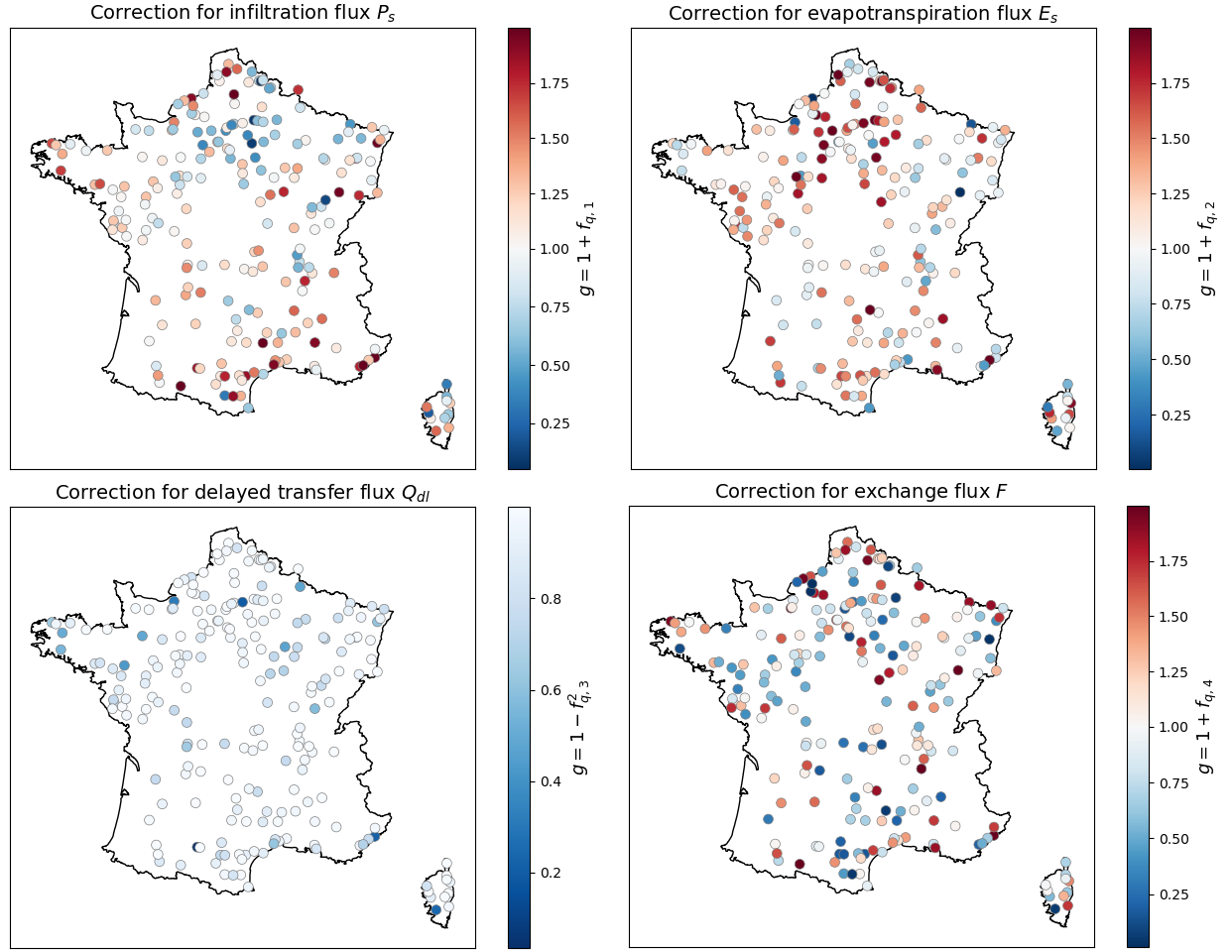
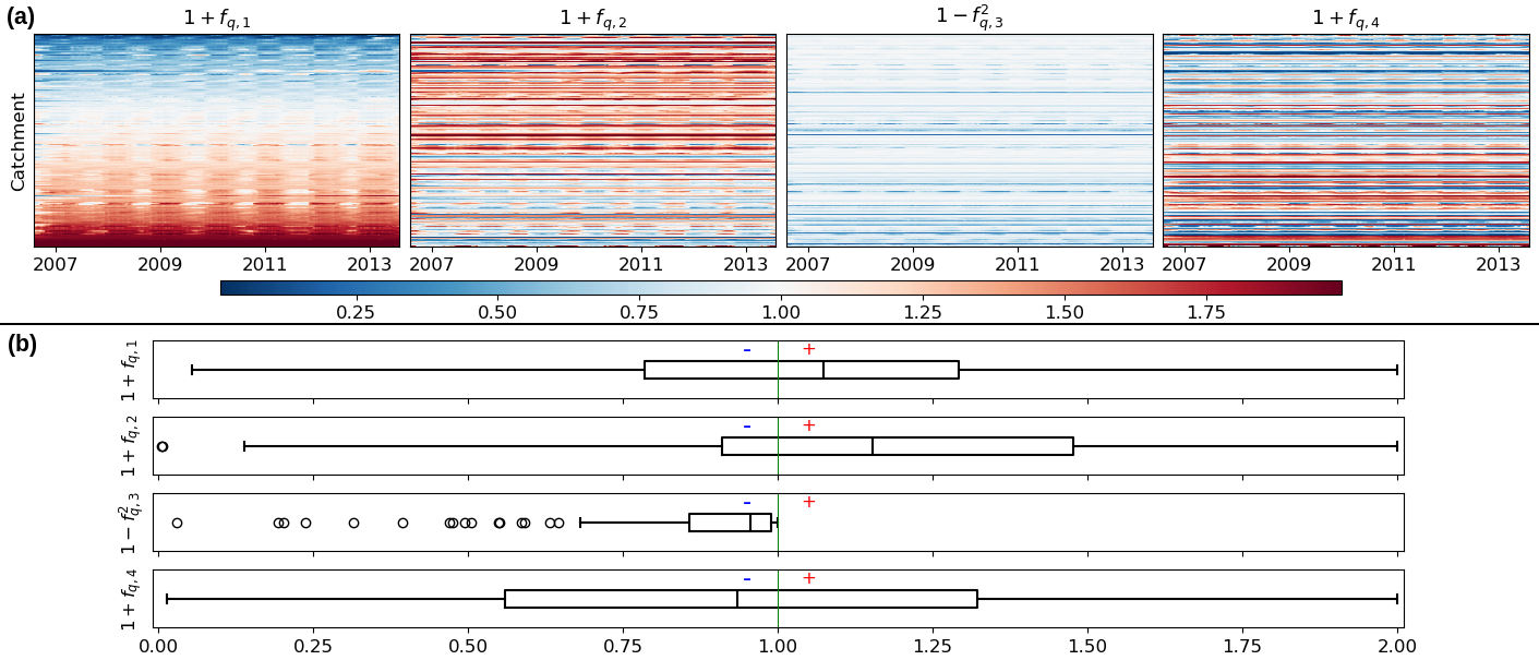
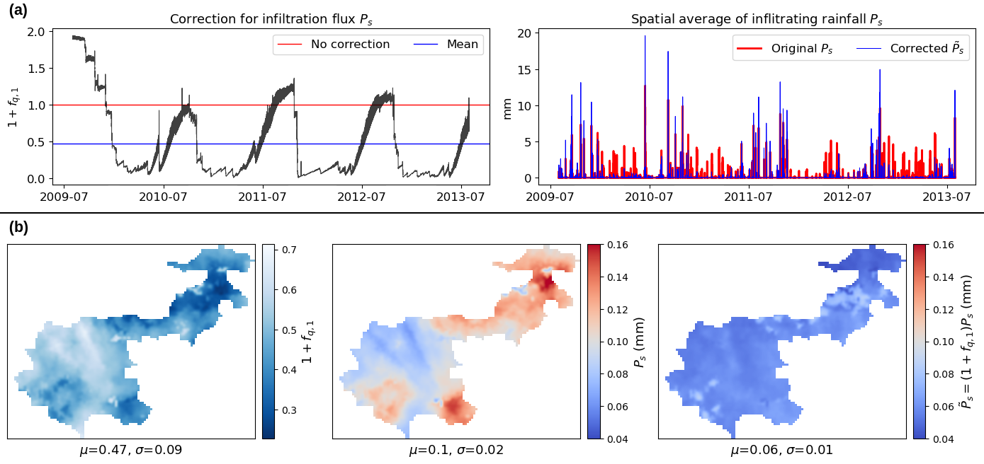
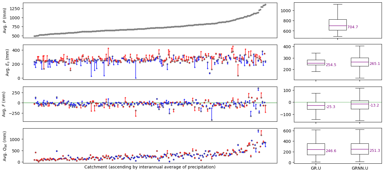
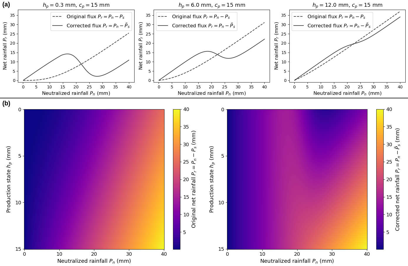
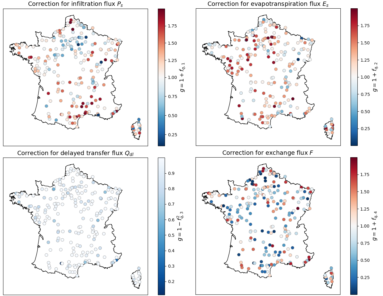
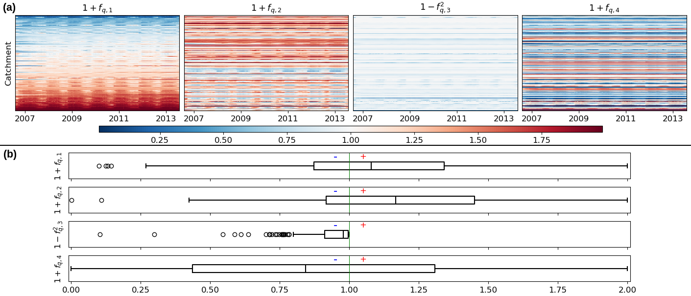
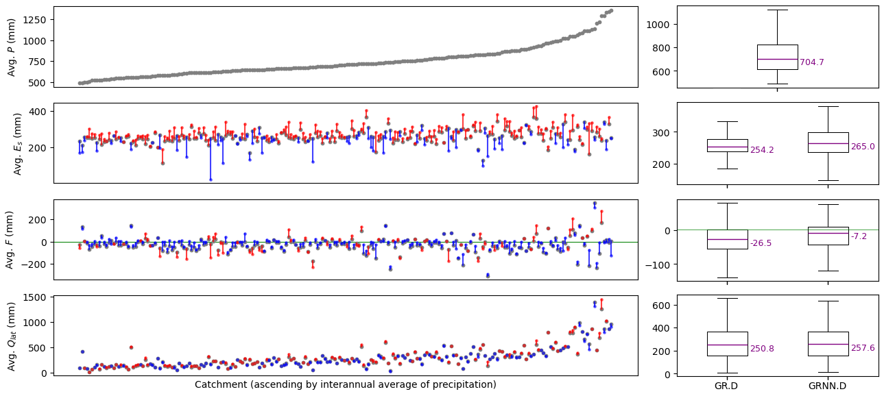
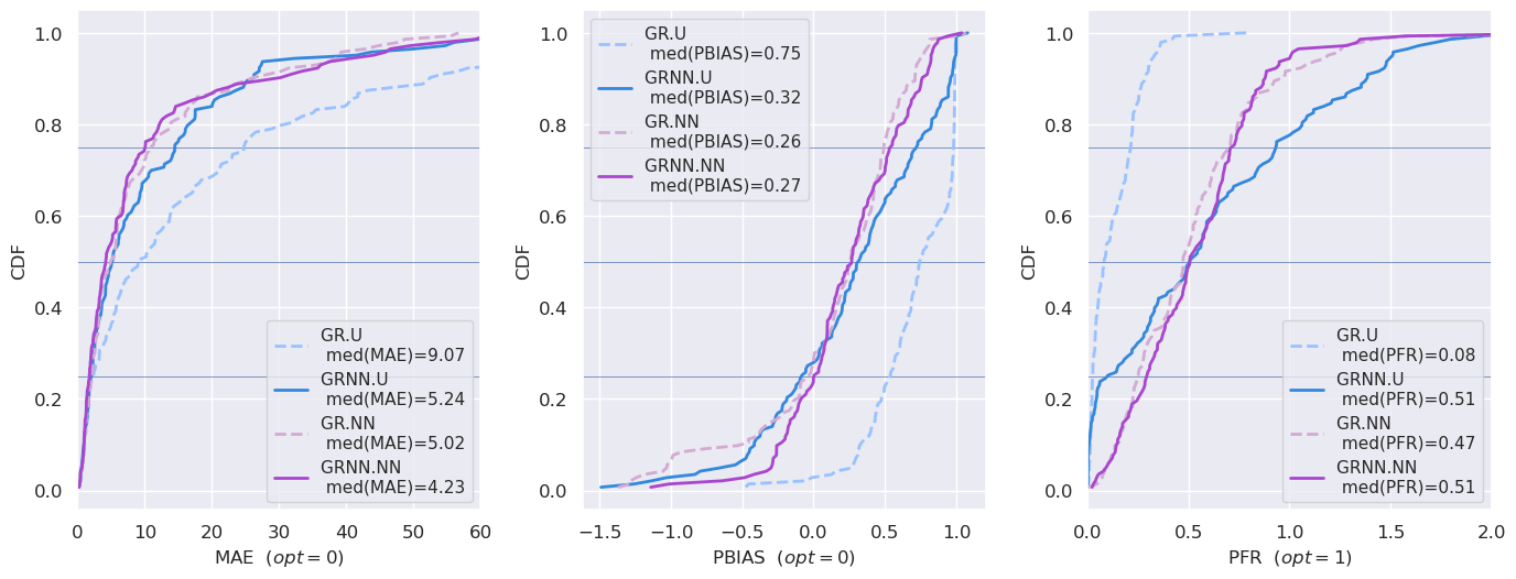
To advance the discovery of scale-relevant hydrological laws while better exploiting massive multisource data, merging artificial intelligence with process-based modeling has emerged as a compelling approach, as demonstrated in recent lumped hydrological modeling studies. This research proposes a general spatially distributed hybrid modeling framework that seamlessly combines differentiable process-based models with neural networks. Specifically, we focus on hybridizing the hydrological module – built atop a differentiable kinematic wave routing over a flow direction grid – using a process-parameterization network that refines internal water fluxes, with all conceptual parameters estimated by a regionalization network trained simultaneously. We evaluate flood modeling performance and analyze the interpretability of learned conceptual parameters and corrections of internal fluxes using two high-resolution datasets (d x =1 km and d t =1 h). The first dataset involves 235 catchments in France, used for local calibration–validation and model structure comparisons between the classical Génie Rural (GR)-like model and the hybrid approach. The second dataset presents a challenging multi-catchment modeling setup in flash-flood-prone areas to demonstrate the framework's regionalization learning capabilities. The results show that the hybrid models achieve superior accuracy and robustness compared to classical approaches in both spatial and temporal validation. Analysis of the spatially distributed parameters and internal fluxes reveals the hybrid models' nuanced behavior, their adaptability to diverse hydrological responses, and their potential to uncover physical processes.
Overview
The claims and statistics of this paper haven’t been checked yet.
Run the check — free, no account needed. It reads the open-access text and checks the sources it cites.
Integrity signals
Registry
Cites
Statistics
Figures
Verification
Claims the paper makes
The claims and statistics of this paper haven’t been checked yet.
Run the check — free, no account needed. It reads the open-access text and checks the sources it cites.
Claims other papers make about this one
Each is checked against this paper’s own text: does it say what the citing paper says it does?
The source backs part of the claim, not all of it — or backs it for a different population, condition or comparison.
In the citing paper
“While the controlled setting of the Yidong Stream strengthens the internal validity of our proof-of-concept, the transferability of this framework to complex meandering or highly urbanized systems requires systematic multi-site evaluation 24 .”
From AI-driven digital twinning quantifies the trade-off between flood conveyance and riparian stability under climate extremes (2026) · cites this paper as [24]
Experimental — accuracy not yet measured
Self-check
Percentages, sums and reported differences re-computed from the paper’s own numbers.
The self-check needs the paper’s full text.
Citations
Cites
Hochreiter, S., & Schmidhuber, J. (1997) · Neural Computation · doi:10.1162/neco.1997.9.8.1735 · Cited by 102,318
LeCun, Y., Bengio, Y., & Hinton, G. (2015) · Nature · doi:10.1038/nature14539 · Cited by 84,126
Neural ordinary differential equations
Chen, R. T. Q., Rubanova, Y., Bettencourt, J., & Duvenaud, D. (2018) · arXiv · doi:10.48550/arxiv.1806.07366 · Cited by 2,097
Research works printed but not linked: 61
- Agency, E. E.: CORINE Land Cover 2012 (raster 100 m), European Environment Agency [data set], 10.2909/a84ae124-c5c5-4577-8e10-511bfe55cc0d, 2019. · DOI
- Arnaud, P., Aubert, Y., Organde, D., Cantet, P., Fouchier, C., and Folton, N.: Estimation de l'aléa hydrométéorologique par une méthode par simulation : la méthode SHYREG : présentation – performances – bases de données, Houille Blanche, 100, 20–26, 10.1051/lhb/2014012, 2014. · DOI
- Artigue, G., Johannet, A., Borrell, V., and Pistre, S.: Flash flood forecasting in poorly gauged basins using neural networks: case study of the Gardon de Mialet basin (southern France), Nat. Hazards Earth Syst. Sci., 12, 3307–3324, 10.5194/nhess-12-3307-2012, 2012. · DOI
- Astagneau, P. C., Bourgin, F., Andréassian, V., and Perrin, C.: When does a parsimonious model fail to simulate floods? Learning from the seasonality of model bias, Hydrolog. Sci. J., 66, 1288–1305, 10.1080/02626667.2021.1923720, 2021. · DOI
- Astagneau, P. C., Bourgin, F., Andréassian, V., and Perrin, C.: Catchment response to intense rainfall: evaluating modelling hypotheses, Hydrol. Process., 36, e14676, 10.1002/hyp.14676, 2022. · DOI
- Brigode, P., Génot, B., Lobligeois, F., and Delaigue, O.: Summary sheets of watershed-scale hydroclimatic observed data for France, Recherche Data Gouv [data set], 10.15454/UV01P1, 2020. · DOI
- Chen, C., Jiang, J., Liao, Z., Zhou, Y., Wang, H., and Pei, Q.: A short-term flood prediction based on spatial deep learning network: a case study for Xi County, China, J. Hydrol., 607, 127535, 10.1016/j.jhydrol.2022.127535, 2022. · DOI
- Colleoni, F., Huynh, N. N. T., Garambois, P.-A., Jay-Allemand, M., Organde, D., Renard, B., De Fournas, T., El Baz, A., Demargne, J., and Javelle, P.: SMASH v1.0: A Differentiable and Regionalizable High-Resolution Hydrological Modeling and Data Assimilation Framework, EGUsphere [preprint], 10.5194/egusphere-2025-690, 2025. · DOI
- Delaigue, O., Guimarães, G. M., Brigode, P., Génot, B., Perrin, C., Soubeyroux, J.-M., Janet, B., Addor, N., and Andréassian, V.: CAMELS-FR dataset: a large-sample hydroclimatic dataset for France to explore hydrological diversity and support model benchmarking, Earth Syst. Sci. Data, 17, 1461–1479, 10.5194/essd-17-1461-2025, 2025. · DOI
- Dooge, J. C. I.: Looking for hydrologic laws, Water Resour. Res., 22, 46S–58S, 10.1029/WR022i09Sp0046S, 1986. · DOI
- Douinot, A., Roux, H., Garambois, P.-A., and Dartus, D.: Using a multi-hypothesis framework to improve the understanding of flow dynamics during flash floods, Hydrol. Earth Syst. Sci., 22, 5317–5340, 10.5194/hess-22-5317-2018, 2018. · DOI
- Feng, D., Liu, J., Lawson, K., and Shen, C.: Differentiable, learnable, regionalized process-based models with multiphysical outputs can approach state-of-the-art hydrologic prediction accuracy, Water Resour. Res., 58, e2022WR032404, 10.1029/2022WR032404, 2022. · DOI
- Ficchì, A., Perrin, C., and Andréassian, V.: Hydrological modelling at multiple sub-daily time steps: model improvement via flux-matching, J. Hydrol., 575, 1308–1327, 10.1016/j.jhydrol.2019.05.084, 2019. · DOI
- Fleischmann, A. S., Paiva, R. C. D., Collischonn, W., Siqueira, V. A., Paris, A., Moreira, D. M., Papa, F., Bitar, A. A., Parrens, M., Aires, F., and Garambois, P. A.: Trade-offs between 1-D and 2-D regional river hydrodynamic models, Water Resour. Res., 56, e2019WR026812, 10.1029/2019WR026812, 2020. · DOI
- Garambois, P.-A., Roux, H., Larnier, K., Labat, D., and Dartus, D.: Parameter regionalization for a process-oriented distributed model dedicated to flash floods, J. Hydrol., 525, 383–399, 2015. · DOI
- Garambois, P.-A., Calmant, S., Roux, H., Paris, A., Monnier, J., Finaud-Guyot, P., Samine Montazem, A., and Santos da Silva, J.: Hydraulic visibility: using satellite altimetry to parameterize a hydraulic model of an ungauged reach of a braided river, Hydrol. Process., 31, 756–767, 10.1002/hyp.11033, 2017. · DOI
- Hascoet, L. and Pascual, V.: The Tapenade automatic differentiation tool: principles, model, and specification, ACM T. Math Software, 39, 1–43, 2013. · DOI
- Hashemi, R., Brigode, P., Garambois, P.-A., and Javelle, P.: How can we benefit from regime information to make more effective use of long short-term memory (LSTM) runoff models?, Hydrol. Earth Syst. Sci., 26, 5793–5816, 10.5194/hess-26-5793-2022, 2022. · DOI
- He, Q., Barajas-Solano, D., Tartakovsky, G., and Tartakovsky, A. M.: Physics-informed neural networks for multiphysics data assimilation with application to subsurface transport, Adv. Water Resour., 141, 103610, 10.1016/j.advwatres.2020.103610, 2020. · DOI
- Höge, M., Scheidegger, A., Baity-Jesi, M., Albert, C., and Fenicia, F.: Improving hydrologic models for predictions and process understanding using neural ODEs, Hydrol. Earth Syst. Sci., 26, 5085–5102, 10.5194/hess-26-5085-2022, 2022. · DOI
- Huynh, N. N. T., Garambois, P.-A., Colleoni, F., and Javelle, P.: Signatures-and-sensitivity-based multi-criteria variational calibration for distributed hydrological modeling applied to Mediterranean floods, J. Hydrol., 625, 129992, 10.1016/j.jhydrol.2023.129992, 2023. · DOI
- Huynh, N. N. T., Garambois, P.-A., Colleoni, F., Renard, B., Monnier, J., and Roux, H.: Multiscale learnable physical modeling and data assimilation framework: application to high-resolution regionalized hydrological simulation of flash flood, Authorea [preprint], 1–26, 10.22541/au.170709054.44271526/v2, 2024a. · DOI
- Huynh, N. N. T., Garambois, P.-A., Colleoni, F., Renard, B., Roux, H., Demargne, J., Jay-Allemand, M., and Javelle, P.: Learning regionalization using accurate spatial cost gradients within a differentiable high-resolution hydrological model: application to the French Mediterranean region, Water Resour. Res., 60, e2024WR037544, 10.1029/2024WR037544, 2024b. · DOI
- Jiang, S., Zheng, Y., and Solomatine, D.: Improving AI system awareness of geoscience knowledge: symbiotic integration of physical approaches and deep learning, Geophys. Res. Lett., 47, e2020GL088229, 10.1029/2020GL088229, 2020. · DOI
- Kingma, D. P. and Ba, J.: Adam: A method for stochastic optimization, arXiv [preprint], 10.48550/arXiv.1412.6980 2014. · DOI · Paper page
- Konapala, G., Kao, S.-C., Painter, S. L., and Lu, D.: Machine learning assisted hybrid models can improve streamflow simulation in diverse catchments across the conterminous US, Environ. Res. Lett., 15, 104022, 10.1088/1748-9326/aba927, 2020. · DOI
- Kratzert, F., Klotz, D., Brenner, C., Schulz, K., and Herrnegger, M.: Rainfall–runoff modelling using Long Short-Term Memory (LSTM) networks, Hydrol. Earth Syst. Sci., 22, 6005–6022, 10.5194/hess-22-6005-2018, 2018. · DOI
- Kratzert, F., Nearing, G., Addor, N., Erickson, T., Gauch, M., Gilon, O., Gudmundsson, L., Hassidim, A., Klotz, D., Nevo, S., Shalev, G., and Matias, Y.: Caravan – a global community dataset for large-sample hydrology, Scientific Data, 10, 61, 10.1038/s41597-023-01975-w, 2023. · DOI
- Kumanlioglu, A. A. and Fistikoglu, O.: Performance enhancement of a conceptual hydrological model by integrating artificial intelligence, J. Hydrol. Eng., 24, 04019047, 10.1061/(ASCE)HE.1943-5584.0001850, 2019. · DOI
- Larnier, K., Garambois, P.-A., Emery, C., Pujol, L., Monnier, J., Gal, L., Paris, A., Yesou, H., Ledauphin, T., and Calmant, S.: Estimating Channel Parameters and Discharge at River Network Scale Using Hydrological-Hydraulic Models, SWOT and Multi-Satellite Data, Water Resour. Res., 61, e2024WR038455, 10.1029/2024WR038455, 2025. · DOI
- Li, B., Sun, T., Tian, F., Tudaji, M., Qin, L., and Ni, G.: Hybrid hydrological modeling for large alpine basins: a semi-distributed approach, Hydrol. Earth Syst. Sci., 28, 4521–4538, 10.5194/hess-28-4521-2024, 2024. · DOI
- Liu, Y. and Gupta, H. V.: Uncertainty in hydrologic modeling: toward an integrated data assimilation framework, Water Resour. Res., 43, W07401, 10.1029/2006WR005756, 2007. · DOI
- Maier, H. R. and Dandy, G. C.: Neural networks for the prediction and forecasting of water resources variables: a review of modelling issues and applications, Environ. Modell. Softw., 15, 101–124, 10.1016/S1364-8152(99)00007-9, 2000. · DOI
- Malou, T., Garambois, P.-A., Paris, A., Monnier, J., and Larnier, K.: Generation and analysis of stage-fall-discharge laws from coupled hydrological-hydraulic river network model integrating sparse multi-satellite data, J. Hydrol., 603, 126993, 10.1016/j.jhydrol.2021.126993, 2021. · DOI
- Meyer Oliveira, A., Fleischmann, A. S., and Paiva, R. C. D.: On the contribution of remote sensing-based calibration to model hydrological and hydraulic processes in tropical regions, J. Hydrol., 597, 126184, 10.1016/j.jhydrol.2021.126184, 2021. · DOI
- Nearing, G. S., Kratzert, F., Sampson, A. K., Pelissier, C. S., Klotz, D., Frame, J. M., Prieto, C., and Gupta, H. V.: What role does hydrological science play in the age of machine learning?, Water Resour. Res., 57, e2020WR028091, 10.1029/2020WR028091, 2021. · DOI · Paper page
- Odry, J.: Prédétermination des débits de crues extrêmes en sites non jaugés : régionalisation de la méthode par simulation SHYREG, PhD thesis, Géosciences de l’environnement, Hydrologie Aix-Marseille 2017, http://www.theses.fr/2017AIXM0424 (last access: 1 August 2025), 2017.
- Organde, D., Arnaud, P., Fine, J.-A., Fouchier, C., Folton, N., and Lavabre, J.: Régionalisation d'une méthode de prédétermination de crue sur l'ensemble du territoire français: la méthode SHYREG, Revue des Sciences de l'Eau, 26, 65–78, 2013. · DOI
- Oudin, L., Hervieu, F., Michel, C., Perrin, C., Andréassian, V., Anctil, F., and Loumagne, C.: Which potential evapotranspiration input for a lumped rainfall–runoff model?: Part 2 Towards a simple and efficient potential evapotranspiration model for rainfall–runoff modelling, J. Hydrol., 303, 290–306, 2005. · DOI
- Oudin, L., Andréassian, V., Perrin, C., Michel, C., and Le Moine, N.: Spatial proximity, physical similarity, regression and ungaged catchments: a comparison of regionalization approaches based on 913 French catchments, Water Resour. Res., 44, W03413, 10.1029/2007WR006240, 2008. · DOI
- Papamarkou, T., Hinkle, J., Young, M. T., and Womble, D.: Challenges in Markov chain Monte Carlo for Bayesian neural networks, Stat. Sci., 37, 425–442, 10.1214/21-STS840, 2022. · DOI
- Perrin, C., Michel, C., and Andrèassian, V.: Improvement of a parsimonious model for streamflow simulation, J. Hydrol., 279, 275–289, 2003. · DOI
- Poncelet, C.: Du bassin au paramètre : jusqu'où peut-on régionaliser un modèle hydrologique conceptuel ?, PhD thesis, Hydrologie Paris 6 2016, http://www.theses.fr/2016PA066550 (last access: 1 August 2025), 2016.
- Pujol, L., Garambois, P.-A., Finaud-Guyot, P., Monnier, J., Larnier, K., Mosé, R., Biancamaria, S., Yesou, H., Moreira, D., Paris, A., and Calmant, S.: Estimation of multiple inflows and effective channel by assimilation of multi-satellite hydraulic signatures: The ungauged anabranching Negro river, J. Hydrol., 591, 125331, 10.1016/j.jhydrol.2020.125331, 2020. · DOI
- Pujol, L., Garambois, P.-A., and Monnier, J.: Multi-dimensional hydrological-hydraulic model with variational data assimilation for river networks and floodplains, EGUsphere [preprint], 10.5194/egusphere-2022-10, 2022. · DOI
- Quintana-Seguí, P., Le Moigne, P., Durand, Y., Martin, E., Habets, F., Baillon, M., Canellas, C., Franchisteguy, L., and Morel, S.: Analysis of near-surface atmospheric variables: validation of the SAFRAN analysis over France, J. Appl. Meteorol. Clim., 47, 92, 10.1175/2007JAMC1636.1, 2008. · DOI
- Rackauckas, C., Ma, Y., Martensen, J., Warner, C., Zubov, K., Supekar, R., Skinner, D., Ramadhan, A., and Edelman, A.: Universal Differential Equations for Scientific Machine Learning, arXiv [preprint], 10.48550/arXiv.2001.04385, 2021. · DOI
- Raissi, M., Perdikaris, P., and Karniadakis, G.: Physics-informed neural networks: a deep learning framework for solving forward and inverse problems involving nonlinear partial differential equations, J. Comput. Phys., 378, 686–707, 10.1016/j.jcp.2018.10.045, 2019. · DOI · Paper page
- Roux, H., Labat, D., Garambois, P.-A., Maubourguet, M.-M., Chorda, J., and Dartus, D.: A physically-based parsimonious hydrological model for flash floods in Mediterranean catchments, Nat. Hazards Earth Syst. Sci., 11, 2567–2582, 10.5194/nhess-11-2567-2011, 2011. · DOI
- Roy, A., Kasiviswanathan, K. S., Patidar, S., Adeloye, A. J., Soundharajan, B.-S., and Ojha, C. S. P.: A novel physics-aware machine learning-based dynamic error correction model for improving streamflow forecast accuracy, Water Resour. Res., 59, e2022WR033318, 10.1029/2022WR033318, 2023. · DOI
- Santos, L., Thirel, G., and Perrin, C.: Continuous state-space representation of a bucket-type rainfall-runoff model: a case study with the GR4 model using state-space GR4 (version 1.0), Geosci. Model Dev., 11, 1591–1605, 10.5194/gmd-11-1591-2018, 2018. · DOI
- Shen, C. and Lawson, K.: Applications of Deep Learning in Hydrology, chap. 19, John Wiley and Sons, Ltd, 10.1002/9781119646181.ch19, 283–297, 2021. · DOI
- Shi, X., Chen, Z., Wang, H., Yeung, D.-Y., Wong, W.-k., and Woo, W.-c.: Convolutional LSTM Network: a machine learning approach for precipitation nowcasting, in: Proceedings of the 28th International Conference on Neural Information Processing Systems – Volume 1, NIPS'15, Montreal, Canada, 7–12 December 2015, 802–810, https://dl.acm.org/doi/10.5555/2969239.2969329 (last access: 1 August 2025), 2015. · DOI
- Tran, V. N., Ivanov, V. Y., Xu, D., and Kim, J.: Closing in on hydrologic predictive accuracy: combining the strengths of high-fidelity and physics-agnostic models, Geophys. Res. Lett., 50, e2023GL104464, 10.1029/2023GL104464, 2023. · DOI
- Tripathy, K. P. and Mishra, A. K.: Deep learning in hydrology and water resources disciplines: concepts, methods, applications, and research directions, J. Hydrol., 628, 130458, 10.1016/j.jhydrol.2023.130458, 2024. · DOI
- Vergara, H., Kirstetter, P.-E., Gourley, J. J., Flamig, Z. L., Hong, Y., Arthur, A., and Kolar, R.: Estimating a-priori kinematic wave model parameters based on regionalization for flash flood forecasting in the Conterminous United States, J. Hydrol., 541, 421–433, 2016. · DOI
- Vidal, J.-P., Martin, E., Franchistéguy, L., Baillon, M., and Soubeyroux, J.-M.: A 50-year high-resolution atmospheric reanalysis over France with the Safran system, Int. J. Climatol., 30, 1627–1644, 10.1002/joc.2003, 2010. · DOI
- Wang, C., Jiang, S., Zheng, Y., Han, F., Kumar, R., Rakovec, O., and Li, S.: Distributed hydrological modeling with physics-encoded deep learning: a general framework and its application in the Amazon, Water Resour. Res., 60, e2023WR036170, 10.1029/2023WR036170, 2024. · DOI
- Xu, T., Longyang, Q., Tyson, C., Zeng, R., and Neilson, B. T.: Hybrid physically based and deep learning modeling of a snow dominated, mountainous, karst watershed, Water Resour. Res., 58, e2021WR030993, 10.1029/2021WR030993, 2022. · DOI
- Yin, Y., Guen, V. L., Dona, J., de Bézenac, E., Ayed, I., Thome, N., and Gallinari, P.: Augmenting physical models with deep networks for complex dynamics forecasting, J. Stat. Mech.-Theory E., 2021, 124012, 10.1088/1742-5468/ac3ae5, 2021. · DOI
- Zhu, C., Byrd, R. H., Lu, P., and Nocedal, J.: Algorithm 778: L-BFGS-B: Fortran subroutines for large-scale bound-constrained optimization, ACM Trans. Math. Softw., 23, 550–560, 1997. · DOI
Cited by
Sorted by citations
Shin, J. H., Go, S. H., & Park, J. H. (2026) · Scientific Reports · doi:10.1038/s41598-026-63704-8
Metadata
- Authors
- Huynh, N. N. T., Garambois, P.-A., Renard, B., Colleoni, F., Monnier, J., & Roux, H.
- Affiliations
- Aix-Marseille Université (FR)
- Institut National des Sciences Appliquées de Toulouse (FR)
- Centre National de la Recherche Scientifique (FR)
- ORCID
- Venue
- Hydrology and Earth System Sciences
- Publisher
- Copernicus GmbH
- Published
- 2025-08-07
- Volume
- 29
- Issue
- 15
- Pages
- 3589-3613
- ISSN
- 1027-5606 (ISSN-L)
- 1607-7938
- OpenAlex
- W4413266363
- Cited by
- 38
- References
- 3
- Citations by year
- 2026: 27 · 2025: 11
- FWCI
- 9.45
- Type
- journal article
- Language
- en
- Open access
- gold
- doi.org
- Licence
- Locations
- Hydrology and earth system sciences (publishedVersion, cc-by)
- HAL (submittedVersion, cc-by)
- HAL (submittedVersion, other-oa)
- DOAJ (DOAJ: Directory of Open Access Journals) (submittedVersion, cc-by-sa)
- Funders
- Agence Nationale de la Recherche (ANR-21-CE04-0021-01)
- Topics
- Physical Sciences › Environmental Science › Environmental Engineering › Hydrological Forecasting Using AI
- Physical Sciences › Environmental Science › Water Science and Technology › Hydrology and Watershed Management Studies
- Physical Sciences › Environmental Science › Global and Planetary Change › Flood Risk Assessment and Management
- Keywords
- distributed hydrological model, kinematic wave routing
About these checks
Registry, retraction, Cites and statistics results are computed, not judged, with one exception: a printed reference that no index lists is read once by a model before it counts as a citation error. Claims are extracted by a model and kept only when their quote appears verbatim in the text; each cited source is then checked, with a model’s help, for whether it says what the claim relies on. Those verdicts can be wrong — read the claim’s quote and the cited source before relying on one.
Statistics and arithmetic are recomputed, not judged.
Confidence bands are shown only for fields calibrated on our annotated test set. None is calibrated yet, so no band is shown.
What counts as a claim ›How we measure confidence ›How we check this ›
Are you an author, or do you see a problem with this page? Request a review
