

The DOI matches its Crossref record; 69 of the 70 references it cites were found in a registry or an index.
A single-embryo, single-cell time-resolved model for mouse gastrulation
Open accessAbstract
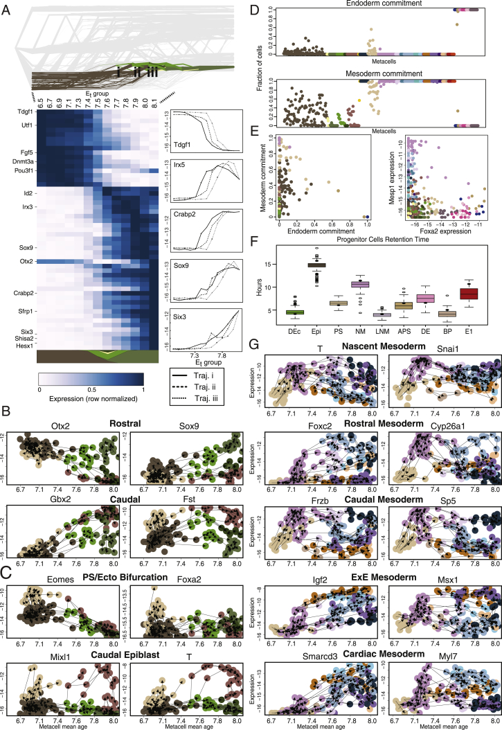
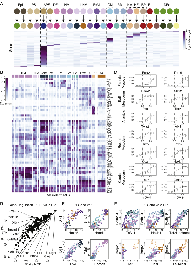
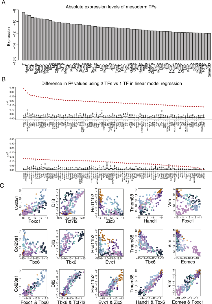
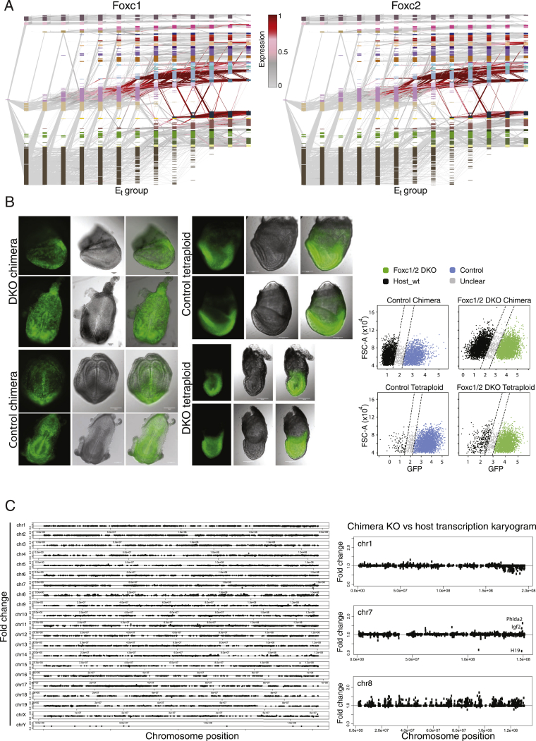
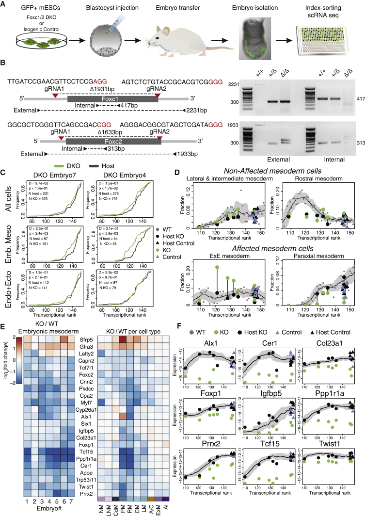
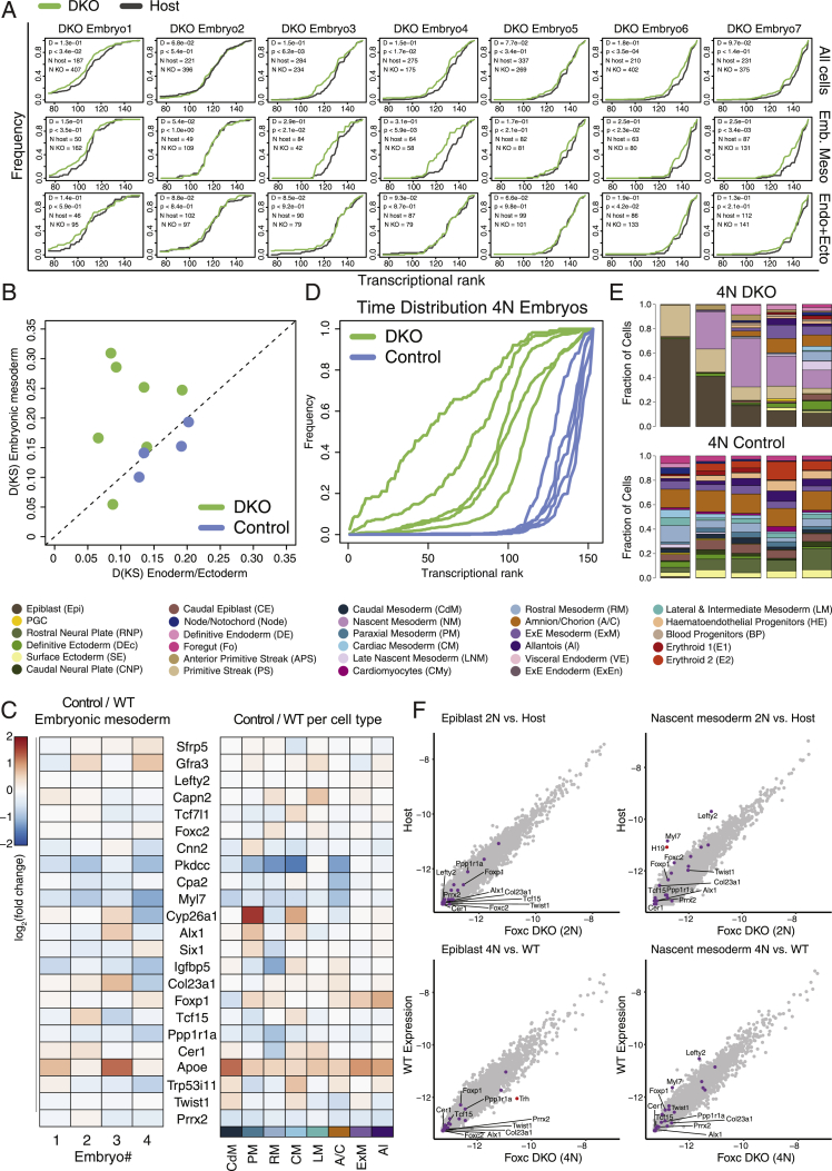
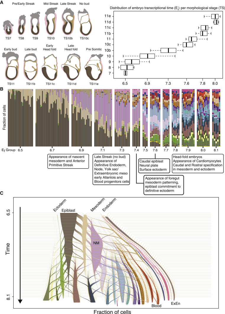
Mouse embryonic development is a canonical model system for studying mammalian cell fate acquisition. Recently, single-cell atlases comprehensively charted embryonic transcriptional landscapes, yet inference of the coordinated dynamics of cells over such atlases remains challenging. Here, we introduce a temporal model for mouse gastrulation, consisting of data from 153 individually sampled embryos spanning 36 h of molecular diversification. Using algorithms and precise timing, we infer differentiation flows and lineage specification dynamics over the embryonic transcriptional manifold. Rapid transcriptional bifurcations characterize the commitment of early specialized node and blood cells. However, for most lineages, we observe combinatorial multi-furcation dynamics rather than hierarchical transcriptional transitions. In the mesoderm, dozens of transcription factors combinatorially regulate multifurcations, as we exemplify using time-matched chimeric embryos of Foxc1/Foxc2 mutants. Our study rejects the notion of differentiation being governed by a series of binary choices, providing an alternative quantitative model for cell fate acquisition.
Overview
The claims and statistics of this paper haven’t been checked yet.
Run the check — free, no account needed. It reads the open-access text and checks the sources it cites.
Integrity signals
Registry
Cites
Statistics
Figures
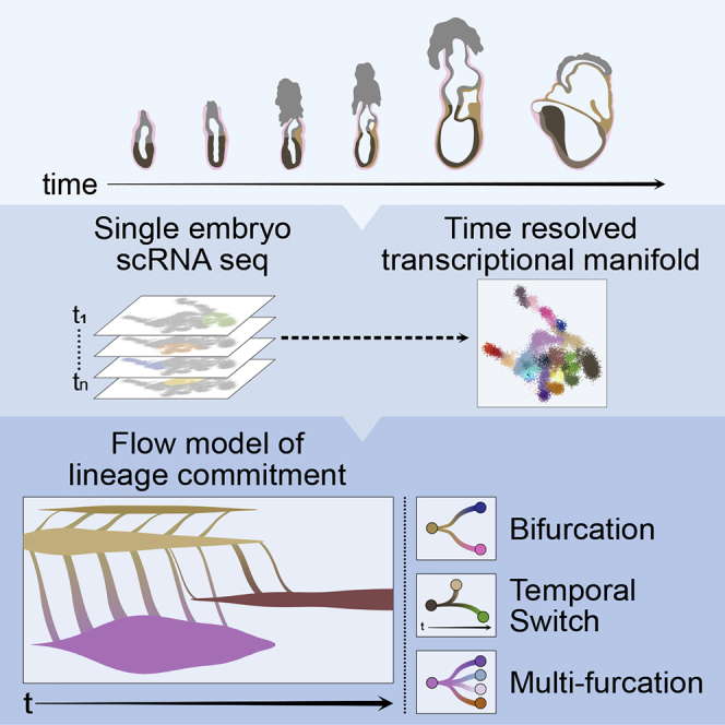
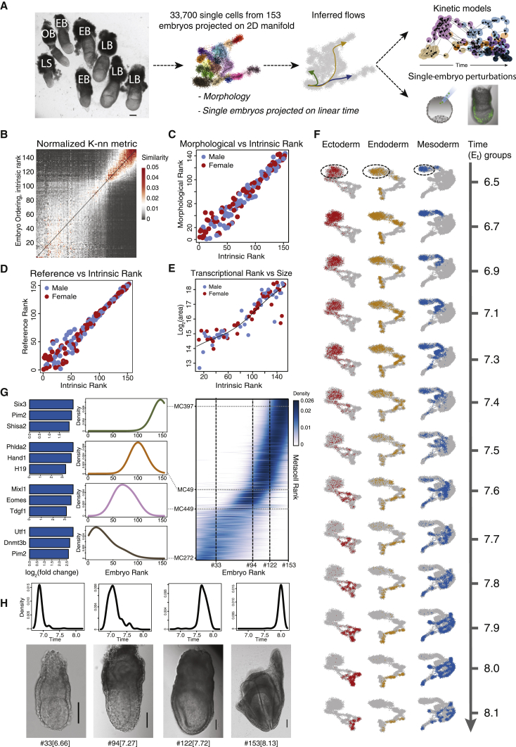
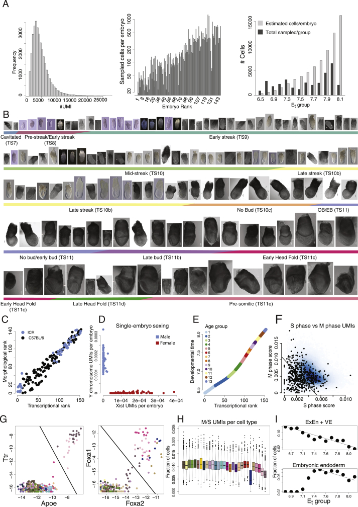
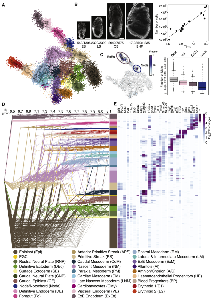
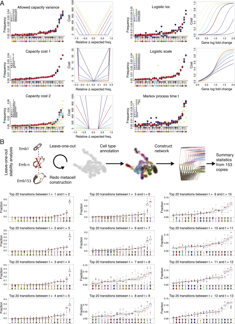
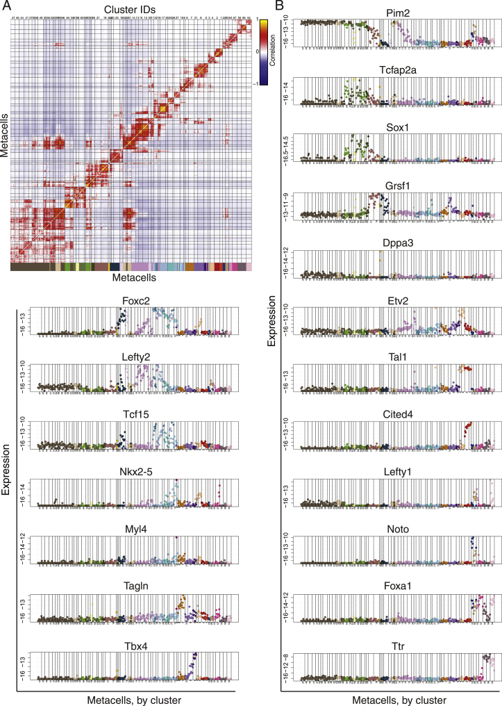
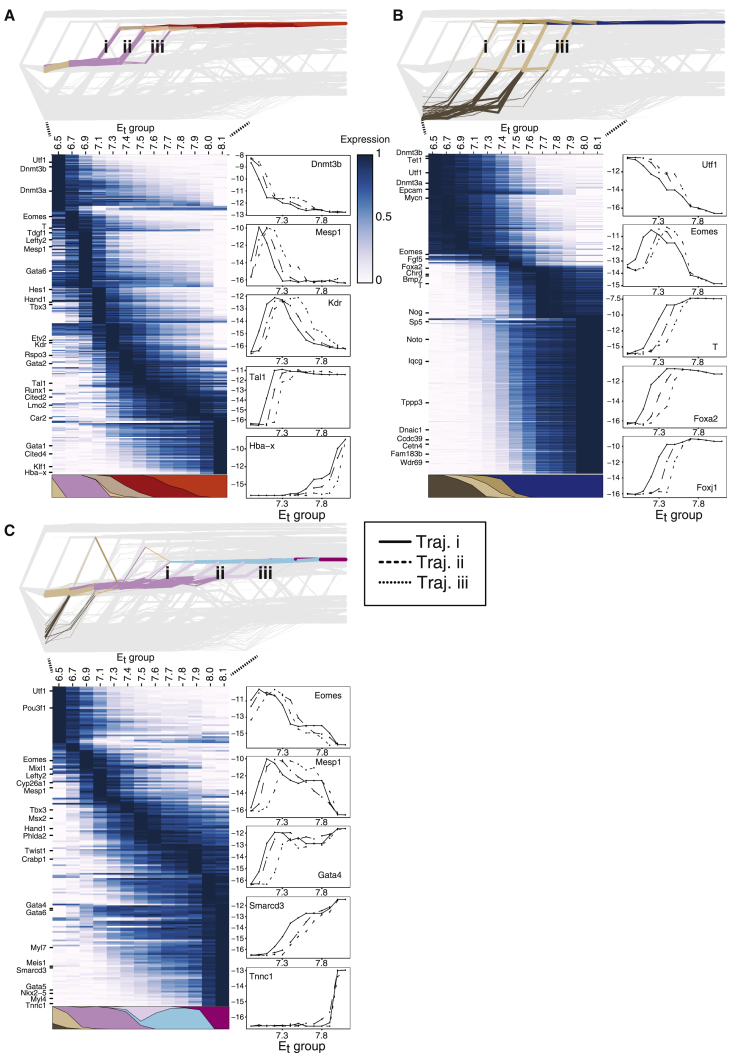
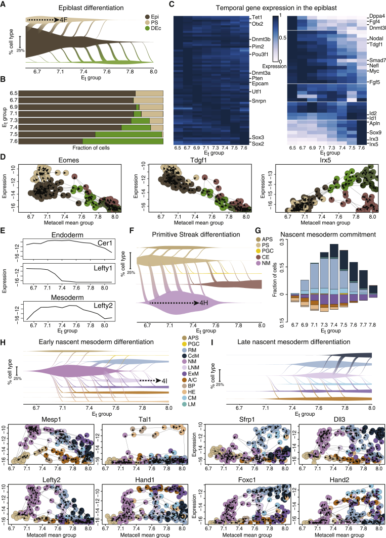
Verification
Claims the paper makes
The claims and statistics of this paper haven’t been checked yet.
Run the check — free, no account needed. It reads the open-access text and checks the sources it cites.
Claims other papers make about this one
Each is checked against this paper’s own text: does it say what the citing paper says it does?
The source backs part of the claim, not all of it — or backs it for a different population, condition or comparison.
In the citing paper
“recent insights into the understanding of cell fate choice, which have suggested a more distributed form of control relying on combinatorial activities of dozens of TFs rather than an organization strictly dominated by a few master TFs (Chubb et al, 2021; Mittnenzweig et al, 2021).”
From An extended transcription factor regulatory network controls hepatocyte identity (2023) · cites this paper as Mittnenzweig et al, 2021
Experimental — accuracy not yet measured
Self-check
Percentages, sums and reported differences re-computed from the paper’s own numbers.
The self-check needs the paper’s full text.
Citations
Cites
Network Flows: Theory, Algorithms, and Applications.
Smith, D. K., Ahuja, R. K., Magnanti, T. L., & Orlin, J. B. (1994) · Journal of the Operational Research Society · doi:10.2307/2583863 · Cited by 8,121
The single-cell transcriptional landscape of mammalian organogenesis
Cao, J., Spielmann, M., Qiu, X., Huang, X., Ibrahim, D. M., Hill, A. J., Zhang, F., Mundlos, S., Christiansen, L., Steemers, F. J., et al. (2019) · Nature · doi:10.1038/s41586-019-0969-x · Cited by 4,490
La Manno, G., Soldatov, R., Zeisel, A., Braun, E., Hochgerner, H., Petukhov, V., Lidschreiber, K., Kastriti, M. E., Lönnerberg, P., Furlan, A., et al. (2018) · Nature · doi:10.1038/s41586-018-0414-6 · Cited by 4,118
Ben‐Porath, I., Thomson, M., Carey, V. J., Ge, R., Bell, G. W., Regev, A., & Weinberg, R. A. (2008) · Nature Genetics · doi:10.1038/ng.127 · Cited by 2,571
New cell lines from mouse epiblast share defining features with human embryonic stem cells
Tesar, P. J., Chenoweth, J. G., Brook, F. A., Davies, T. J., Evans, E. P., Mack, D. L., Gardner, R. L., & McKay, R. D. G. (2007) · Nature · doi:10.1038/nature05972 · Cited by 2,187
Derivation of pluripotent epiblast stem cells from mammalian embryos
Brons, I. G. M., Smithers, L. E., Trotter, M. W. B., Rugg‐Gunn, P. J., Sun, B., Lopes, S. M. C. D. S., Howlett, S., Clarkson, A., Ährlund‐Richter, L., Pedersen, R. A., et al. (2007) · Nature · doi:10.1038/nature05950 · Cited by 2,007
Massively parallel single-cell RNA-seq for marker-free decomposition of tissues into cell types
Jaitin, D. A., Kenigsberg, E., Keren-Shaul, H., Elefant, N., Paul, F., Zaretsky, I., Mildner, A., Cohen, N., Jung, S., Tanay, A., et al. (2014) · Science · doi:10.1126/science.1247651 · Cited by 1,795
Self-citationMapping the Mouse Cell Atlas by Microwell-Seq
Han, X., Wang, R., Zhou, Y., Fei, L., Sun, H., Lai, S., Saadatpour, A., Zhou, Z., Chen, H., Ye, F., et al. (2018) · Cell · doi:10.1016/j.cell.2018.02.001 · Cited by 1,597
Development of erythroid and myeloid progenitors in the yolk sac and embryo proper of the mouse
Palis, J., Robertson, S. M., Kennedy, M., Wall, C., & Keller, G. M. (1999) · Development · doi:10.1242/dev.126.22.5073 · Cited by 1,093
CCTop: An intuitive, flexible and reliable CRISPR/Cas9 target prediction tool
Stemmer, M., Thumberger, T., del Sol Keyer, M., Wittbrodt, J., & Mateo, J. L. (2015) · PLoS ONE · doi:10.1371/journal.pone.0124633 · Cited by 1,088
Cited by
Sorted by citations
Inferring and perturbing cell fate regulomes in human brain organoids
Fleck, J. S., Jansen, S. M. J., Wollny, D., Zenk, F., Seimiya, M., Jain, A., Okamoto, R., Santel, M., He, Z., Camp, J. G., et al. (2023) · Nature · doi:10.1038/s41586-022-05279-8 · Cited by 315
Post-gastrulation synthetic embryos generated ex utero from mouse naive ESCs
Tarazi, S., Aguilera-Castrejon, A., Joubran, C., Ghanem, N., Ashouokhi, S., Roncato, F., Wildschutz, E., Haddad, M., Oldak, B., Gomez-Cesar, E., et al. (2022) · Cell · doi:10.1016/j.cell.2022.07.028 · Cited by 246
Herring, C. A., Simmons, R. K., Freytag, S., Poppe, D., Moffet, J. J. D., Pflueger, J., Buckberry, S., Vargas-Landín, D. B., Clément, O., Goñi, E., et al. (2022) · Cell · doi:10.1016/j.cell.2022.09.039 · Cited by 242
High-throughput total RNA sequencing in single cells using VASA-seq
Salmén, F., Jonghe, J. D., Kamiński, T. S., Alemany, A., Parada, G. E., Verity-Legg, J., Yanagida, A., Kohler, T. N., Battich, N., van den Brekel, F., et al. (2022) · Nature Biotechnology · doi:10.1038/s41587-022-01361-8 · Cited by 244
A single-cell time-lapse of mouse prenatal development from gastrula to birth
Qiu, C., Martin, B., Welsh, I. C., Daza, R. M., Le, T.-M., Huang, X., Nichols, E. K., Taylor, M. L., Fulton, O., O’Day, D. R., et al. (2024) · Nature · doi:10.1038/s41586-024-07069-w · Cited by 215
A reference cell tree will serve science better than a reference cell atlas
Domcke, S., & Shendure, J. (2023) · Cell · doi:10.1016/j.cell.2023.02.016 · Cited by 113
Lau, K. Y. C., Rubinstein, H., Gantner, C. W., Hadas, R., Amadei, G., Stelzer, Y., & Zernicka‐Goetz, M. (2022) · Cell stem cell · doi:10.1016/j.stem.2022.08.013 · Cited by 114
Self-citationFei, L., Chen, H., Ma, L., Weigao, E., Wang, R., Fang, X., Zhou, Z., Sun, H., Wang, J., Jiang, M., et al. (2022) · Nature Genetics · doi:10.1038/s41588-022-01118-8 · Cited by 114
Primate gastrulation and early organogenesis at single-cell resolution
Zhai, J., Guo, J., Wan, H., Qi, L. Q. L., Liu, L., Xiao, Z., Long, Y., Schmitz, D. A., Xu, Y., Yu, D., et al. (2022) · Nature · doi:10.1038/s41586-022-05526-y · Cited by 106
The continuum of Drosophila embryonic development at single-cell resolution
Calderon, D., Blecher‐Gonen, R., Huang, X., Secchia, S., Kentro, J. A., Daza, R. M., Martin, B., Dulja, A., Schaub, C., Trapnell, C., et al. (2022) · Science · doi:10.1126/science.abn5800 · Cited by 100
Deep-tissue transcriptomics and subcellular imaging at high spatial resolution
Gandin, V., Kim, J., Yang, L.-Z., Lian, Y., Kawase, T., Hu, A., Rokicki, K., Fleishman, G. M., Tillberg, P. W., Aguilera-Castrejon, A., et al. (2025) · Science · doi:10.1126/science.adq2084 · Cited by 105
Connecting past and present: single-cell lineage tracing
Chen, C., Liao, Y., & Peng, G. (2022) · Protein & Cell · doi:10.1007/s13238-022-00913-7 · Cited by 99
Modelling post-implantation human development to yolk sac blood emergence
Hislop, J., Song, Q., Kamyar Keshavarz, F., Alavi, A., Schoenberger, R., LeGraw, R., Velazquez, J. J., Mokhtari, T., Taheri, M. N., Rytel, M., et al. (2023) · Nature · doi:10.1038/s41586-023-06914-8 · Cited by 96
Hallmarks of totipotent and pluripotent stem cell states
Du, P., & Wu, J. (2024) · Cell stem cell · doi:10.1016/j.stem.2024.01.009 · Cited by 92
Pera, M. F., & Rossant, J. (2021) · Cell stem cell · doi:10.1016/j.stem.2021.10.001 · Cited by 86
Optimal transport for single-cell and spatial omics
Bunne, C., Schiebinger, G., Krause, A., Regev, A., & Cuturi, M. (2024) · Nature Reviews Methods Primers · doi:10.1038/s43586-024-00334-2 · Cited by 71
Advances and applications in single-cell and spatial genomics
Wang, J., Ye, F., Chai, H., Jiang, Y., Wang, T., Ran, X., Xia, Q., Xu, Z., Fu, Y., Zhang, G., et al. (2024) · Science China Life Sciences · doi:10.1007/s11427-024-2770-x · Cited by 70
Neurulation of the cynomolgus monkey embryo achieved from 3D blastocyst culture
Zhai, J., Xu, Y., Wan, H., Yan, R., Guo, J., Skory, R. M., Long, Y., Wu, X., Sun, F., Chen, G., et al. (2023) · Cell · doi:10.1016/j.cell.2023.04.019 · Cited by 63
Precise and scalable self-organization in mammalian pseudo-embryos
Merle, M., Friedman, L., Chureau, C., Shoushtarizadeh, A., & Gregor, T. (2024) · Nature Structural & Molecular Biology · doi:10.1038/s41594-024-01251-4 · Cited by 53
Murphy, D., Salataj, E., Giammartino, D. C. D., Rodriguez-Hernaez, J., Kloetgen, A., Garg, V., Char, E., Uyehara, C. M., Ee, L.-S., Lee, U., et al. (2023) · Nature Structural & Molecular Biology · doi:10.1038/s41594-023-01130-4 · Cited by 51
Thompson, J. J., Lee, D. J., Mitra, A., Frail, S., Dale, R., & Rocha, P. P. (2022) · Nature Communications · doi:10.1038/s41467-022-31938-5 · Cited by 48
Mapping cells through time and space with moscotPreprint
Klein, D., Palla, G., Lange, M., Klein, M., Piran, Z., Gander, M., Meng-Papaxanthos, L., Sterr, M., Bastidas-Ponce, A., Tarquis-Medina, M., et al. (2023) · bioRxiv (Cold Spring Harbor Laboratory) · doi:10.1101/2023.05.11.540374 · Cited by 49
H3K36 methylation maintains cell identity by regulating opposing lineage programmes
Hoetker, M. S., Yagi, M., Stefano, B. D., Langerman, J., Cristea, S., Wong, L. P., Huebner, A. J., Charlton, J., Deng, W., Haggerty, C., et al. (2023) · Nature Cell Biology · doi:10.1038/s41556-023-01191-z · Cited by 46
The transcriptional portraits of the neural crest at the individual cell level
Erickson, A. G., Kameneva, P., & Adameyko, I. I. (2022) · Seminars in Cell and Developmental Biology · doi:10.1016/j.semcdb.2022.02.017 · Cited by 51
The Intrinsic and Extrinsic Effects of Tet Proteins During Gastrulation
Cheng, S., Mittnenzweig, M., Mayshar, Y., Lifshitz, A., Dunjić, M., Rais, Y., Ben-Yair, R., Gehrs, S., Chomsky, E., Mukamel, Z., et al. (2021) · Cell · doi:10.1016/j.cell.2022.06.049 · Cited by 43
Self-citationFang, W., Bell, C. M., Sapirstein, A., Asami, S., Leeper, K., Zack, D. J., Ji, H., & Kalhor, R. (2022) · Cell · doi:10.1016/j.cell.2022.10.028 · Cited by 44
Single-cell, whole-embryo phenotyping of mammalian developmental disorders
Huang, X., Henck, J., Qiu, C., Sreenivasan, V. K. A., Balachandran, S., Amarie, O. V., de Angelis, M. H., Behncke, R. Y., Chan, W.-L., Despang, A., et al. (2023) · Nature · doi:10.1038/s41586-023-06548-w · Cited by 46
Imaz-Rosshandler, I., Rode, C., Guibentif, C., Harland, L. T. G., Ton, M.-L. N., Dhapola, P., Keitley, D., Argelaguet, R., Calero‐Nieto, F. J., Nichols, J., et al. (2023) · Development · doi:10.1242/dev.201867 · Cited by 41
The heart field transcriptional landscape at single-cell resolution
Kelly, R. G. (2023) · Developmental Cell · doi:10.1016/j.devcel.2023.01.010 · Cited by 39
Pajanoja, C., Hsin, J., Olinger, B., Schiffmacher, A. T., Yazejian, R. M., Abrams, S. R., Dapkunas, A., Zainul, Z., Doyle, A. D., Martı́n, D., et al. (2023) · Nature Communications · doi:10.1038/s41467-023-41384-6 · Cited by 37
The Advancement and Application of the Single-Cell Transcriptome in Biological and Medical Research
Huang, K., Xu, Y., Feng, T., Lan, H., Ling, F., Xiang, H., & Liu, Q. (2024) · Biology · doi:10.3390/biology13060451 · Cited by 44
López-Anguita, N., Gassaloglu, S. I., Stötzel, M., Typou, M., Virta, I., Hetzel, S., Buschow, R., Koksal, B., Atilla, D., Maitschke-Rajasekharan, R., et al. (2022) · Development · doi:10.1242/dev.200679 · Cited by 40
Single-cell transcriptomic characterization of sheep conceptus elongation and implantation
Jia, G., Ma, W., Wu, Z.-B., Li, S., Zhang, X., He, Z., Wu, S., Tao, H.-P., Fang, Y., Song, Y.-W., et al. (2023) · Cell Reports · doi:10.1016/j.celrep.2023.112860 · Cited by 39
Quantifying cell-state densities in single-cell phenotypic landscapes using Mellon
Otto, D. J., Jordan, C., Dury, B., Dien, C., & Setty, M. N. (2024) · Nature Methods · doi:10.1038/s41592-024-02302-w · Cited by 38
Vianello, S., & Lütolf, M. P. (2020) · bioRxiv (Cold Spring Harbor Laboratory) · doi:10.1101/2020.06.07.138883 · Cited by 38
Cell lineage-specific mitochondrial resilience during mammalian organogenesis
Burr, S. P., Klimm, F., Glynos, A., Prater, M., Sendon, P., Nash, P. A., Powell, C. A., Simard, M., Bonekamp, N. A., Charl, J., et al. (2023) · Cell · doi:10.1016/j.cell.2023.01.034 · Cited by 36
Time-aligned hourglass gastrulation models in rabbit and mouse
Mayshar, Y., Raz, O., Cheng, S., Ben-Yair, R., Hadas, R., Reines, N., Mittnenzweig, M., Ben-Kiki, O., Lifshitz, A., Tanay, A., et al. (2023) · Cell · doi:10.1016/j.cell.2023.04.037 · Cited by 34
Self-citationSpatial and Molecular Anatomy of Germ Layers in the Gastrulating Cynomolgus Monkey Embryo
Cui, G., Feng, S., Yan, Y., Wang, L., He, X., Li, X., Duan, Y., Chen, J., Tang, K., Zheng, P., et al. (2022) · Cell Reports · doi:10.1016/j.celrep.2022.111285 · Cited by 34
Inferring and perturbing cell fate regulomes in human cerebral organoidsPreprint
Fleck, J. S., Jansen, S. M. J., Wollny, D., Seimiya, M., Zenk, F. L., Santel, M., He, Z., Camp, J. G., & Treutlein, B. (2021) · bioRxiv (Cold Spring Harbor Laboratory) · doi:10.1101/2021.08.24.457460 · Cited by 35
Single-cell multi-omics and lineage tracing to dissect cell fate decision-making
Haghverdi, L., & Ludwig, L. S. (2023) · Stem Cell Reports · doi:10.1016/j.stemcr.2022.12.003 · Cited by 37
Li, T., Zou, Y., Liu, S., Yang, Y. A., Zhang, Z., & Zhao, Y. (2022) · Cell Regeneration · doi:10.1186/s13619-021-00105-4 · Cited by 35
Approaches for single-cell RNA sequencing across tissues and cell types
Sant, P., Rippe, K., & Mallm, J. (2023) · Transcription · doi:10.1080/21541264.2023.2200721 · Cited by 34
The development of the amnion in mice and other amniotes
Lopes, S. M. C. D. S., Roelen, B. A. J., Lawson, K. A., & Zwijsen, A. (2022) · Philosophical Transactions of the Royal Society B Biological Sciences · doi:10.1098/rstb.2021.0258 · Cited by 31
Temporal BMP4 effects on mouse embryonic and extraembryonic development
Hadas, R., Rubinstein, H., Mittnenzweig, M., Mayshar, Y., Ben-Yair, R., Cheng, S., Aguilera-Castrejon, A., Reines, N., Orenbuch, A.-H., Lifshitz, A., et al. (2024) · Nature · doi:10.1038/s41586-024-07937-5 · Cited by 32
Self-citationRosen, L. U., Stapel, L. C., Argelaguet, R., Barker, C. G., Yang, A., Reik, W., & Marioni, J. C. (2022) · bioRxiv (Cold Spring Harbor Laboratory) · doi:10.1101/2022.09.27.509783 · Cited by 28
Yang, X. H., Goldstein, A., Sun, Y., Wang, Z., Wei, M., Moskowitz, I. P. G., & Cunningham, J. M. (2022) · Nucleic Acids Research · doi:10.1093/nar/gkac452 · Cited by 28
Maizels, R. J., Snell, D. M., & Briscoe, J. (2024) · Cell Systems · doi:10.1016/j.cels.2024.04.004 · Cited by 36
Juvenile hormone as a key regulator for asymmetric caste differentiation in ants
Li, R., Dai, X., Zheng, J., Larsen, R. S., Qi, Y., Zhang, X., Vizueta, J., Boomsma, J. J., Liu, W., & Zhang, G. (2024) · Proceedings of the National Academy of Sciences · doi:10.1073/pnas.2406999121 · Cited by 34
A single-cell atlas of pig gastrulation as a resource for comparative embryology
Simpson, L., Strange, A., Klisch, D., Kraunsoe, S., Azami, T., Goszczynski, D. E., Minh, T. L., Planells, B., Holmes, N., Sang, F., et al. (2024) · Nature Communications · doi:10.1038/s41467-024-49407-6 · Cited by 33
Proks, M., Salehin, N., & Brickman, J. M. (2024) · Nature Methods · doi:10.1038/s41592-024-02511-3 · Cited by 32
Fetal Leydig cells: What we know and what we don't
Jiang, K., & Jorgensen, J. S. (2024) · Molecular Reproduction and Development · doi:10.1002/mrd.23739 · Cited by 32
Tyshkovskiy, A., Kholdina, D., Ying, K., Davitadze, M., Molière, A., Tongu, Y., Kasahara, T., Kats, L., Vladimirova, A., Moldakozhayev, A., et al. (2024) · bioRxiv (Cold Spring Harbor Laboratory) · doi:10.1101/2024.07.04.601982 · Cited by 32
Actin polymerization and depolymerization in developing vertebrates
Bai, Y., Zhao, F., Wu, T., Chen, F., & Pang, X. (2023) · Frontiers in Physiology · doi:10.3389/fphys.2023.1213668 · Cited by 31
Thowfeequ, S., Fiorentino, J., Hu, D., Solovey, M., Ruane, S., Whitehead, M. A., Zhou, F., Godwin, J., Mateo‐Otero, Y., Vanhaesebroeck, B., et al. (2024) · Developmental Cell · doi:10.1016/j.devcel.2024.05.014 · Cited by 25
Dissecting mammalian reproduction with spatial transcriptomics
Zhang, X., Cao, Q., Rajachandran, S., Grow, E. J., Evans, M., & Chen, H. (2023) · Human Reproduction Update · doi:10.1093/humupd/dmad017 · Cited by 25
Hopkins, B. R., Barmina, O. Y., & Kopp, A. (2023) · PLoS Biology · doi:10.1371/journal.pbio.3002148 · Cited by 24
Atoh8 in Development and Disease
Divvela, S. S. K., Saberi, D., & Brand‐Saberi, B. (2022) · Biology · doi:10.3390/biology11010136 · Cited by 22
Balanced gene dosage control rather than parental origin underpins genomic imprinting
Weinberg‐Shukron, A., Ben-Yair, R., Takahashi, N., Dunjić, M., Shtrikman, A., Edwards, C. A., Ferguson‐Smith, A. C., & Stelzer, Y. (2022) · Nature Communications · doi:10.1038/s41467-022-32144-z · Cited by 21
Self-citationCohesin prevents cross-domain gene coactivation
Dong, P., Zhang, S., Gandin, V., Xie, L., Wang, L., Lemire, A. L., Li, W., Otsuna, H., Kawase, T., Lander, A. D., et al. (2024) · Nature Genetics · doi:10.1038/s41588-024-01852-1 · Cited by 26
Three‐dimensional stem cell models of mammalian gastrulation
Turner, D. A., & Arias, A. M. (2024) · BioEssays · doi:10.1002/bies.202400123 · Cited by 19
Swift, J., Greenham, K., Ecker, J. R., Coruzzi, G. M., & McClung, C. R. (2021) · The Plant Journal · doi:10.1111/tpj.15589 · Cited by 22
Digital reconstruction of full embryos during early mouse organogenesis
Xie, P., Shen, J., Yang, Y., Wang, X., Liu, W., Cao, H., Zheng, Y., Wu, C., Mao, G., He, J., et al. (2025) · Cell · doi:10.1016/j.cell.2025.05.035 · Cited by 21
Nox4 promotes endothelial differentiation through chromatin remodeling
Hahner, F., Moll, F., Warwick, T., Hebchen, D. M., Buchmann, G., Epah, J., Abplanalp, W. T., Schader, T., Günther, S., Gilsbach, R., et al. (2022) · Redox Biology · doi:10.1016/j.redox.2022.102381 · Cited by 19
LoxCode in vivo barcoding reveals epiblast clonal fate bias to fetal organs
Weber, T., Biben, C., Miles, D. C., Glaser, S. P., Tomei, S., Lin, C., Kueh, A. J., Pál, M., Zhang, S., Tam, P., et al. (2025) · Cell · doi:10.1016/j.cell.2025.04.026 · Cited by 26
Guo, X., Ning, J., Chen, Y., Liu, G., Zhao, L., Fan, Y., & Sun, S. (2023) · Briefings in Functional Genomics · doi:10.1093/bfgp/elad011 · Cited by 19
Building and analyzing metacells in single-cell genomics data
Bilous, M., Hérault, L., Gabriel, A. A., Teleman, M., & Gfeller, D. (2024) · Molecular Systems Biology · doi:10.1038/s44320-024-00045-6 · Cited by 18
Yılmaz, A., Gurhan, G., Comar, M.-Y., Viukov, S. V., Serfaty, I., Gayretli, M., Golenchenko, S., Lokshtanov, D., Ashouokhi, S., Polanco, A., et al. (2025) · Cell Stem Cell · doi:10.1016/j.stem.2025.07.005 · Cited by 15
Self-citationQi, S., Wang, W., Xue, X., Zhuo, L., Yan, J., Li, Y., Zhang, Y., Shu, M., Song, C., Wang, Q., et al. (2022) · PLoS Biology · doi:10.1371/journal.pbio.3001741 · Cited by 17
The extended analogy of extraembryonic development in insects and amniotes
Panfilio, K. A., & Lopes, S. M. C. D. S. (2022) · Philosophical Transactions of the Royal Society B Biological Sciences · doi:10.1098/rstb.2021.0268 · Cited by 17
exFINDER: identify external communication signals using single-cell transcriptomics data
He, C., Zhou, P., & Nie, Q. H. (2023) · Nucleic Acids Research · doi:10.1093/nar/gkad262 · Cited by 17
Zhang, H., Nie, J., Bao, Z., Shi, Y., Gong, J., & Li, H. (2025) · Cellular Signalling · doi:10.1016/j.cellsig.2025.111680 · Cited by 17
Oka, S., Tsuzuki, T., Hidaka, M., Ohno, M., Nakatsu, Y., & Sekiguchi, M. (2022) · Cell Death Discovery · doi:10.1038/s41420-022-00961-2 · Cited by 16
Icaritin inhibits endometrial carcinoma cells by suppressing O-GlcNAcylation of FOXC1
Wang, Y., Wang, G., Liu, Y., Yang, F., Zhang, H., & Kong, Y. (2023) · Phytomedicine · doi:10.1016/j.phymed.2023.155062 · Cited by 16
A synthetic differentiation circuit in Escherichia coli for suppressing mutant takeover
Glass, D. S., Bren, A., Vaisbourd, E., Mayo, A., & Alon, U. S. (2024) · Cell · doi:10.1016/j.cell.2024.01.024 · Cited by 14
Chugunov, A. O., Potapova, N. A., Klimenko, N. S., Tatarskiy, V. V., Georgieva, S. G., & Soshnikova, N. V. (2021) · International Journal of Molecular Sciences · doi:10.3390/ijms222011134 · Cited by 15
Gene regulatory networks: from correlative models to causal explanations
Maizels, R. J., & Briscoe, J. (2026) · Nature Reviews Genetics · doi:10.1038/s41576-026-00939-1 · Cited by 21
Guan, G., Li, Z., Ma, Y., Ye, P., Cao, J., Wong, M., Ho, V. W. S., Chan, L.-Y., Yan, H., Tang, C., et al. (2025) · Nature Communications · doi:10.1038/s41467-025-58878-0 · Cited by 14
Harland, L. T. G., Lohoff, T., Koulena, N., Pierson, N. G., Pape, C., Ameen, F., Griffiths, J. A., Theeuwes, B., Wilson, N. K., Kreshuk, A., et al. (2025) · Cell Reports · doi:10.1016/j.celrep.2025.116047 · Cited by 13
Stem Cell and Synthetic Embryo Models: Advances, Applications, and Ethical Considerations
Marei, H. E. S. (2025) · Stem Cell Reviews and Reports · doi:10.1007/s12015-025-10890-z · Cited by 14
Dissecting the Complexity of Early Heart Progenitor Cells
Sendra, M., Dominguez, J. N., Torres, M., & Ocaña, O. H. (2021) · Journal of Cardiovascular Development and Disease · doi:10.3390/jcdd9010005 · Cited by 16
Transient upregulation of IRF1 during exit from naive pluripotency confers viral protection
Romeike, M., Spach, S., Huber, M. L., Feng, S., Vainorius, G., Elling, U., Versteeg, G. A., & Buecker, C. (2022) · EMBO Reports · doi:10.15252/embr.202255375 · Cited by 13
van der Veer, B. K., Chen, L., Custers, C., Athanasouli, P., Schroiff, M., Cornelis, R., Chui, J. S., Finnell, R. H., Lluís, F., & Koh, K. P. (2023) · Nucleic Acids Research · doi:10.1093/nar/gkad231 · Cited by 17
The evolving definition of plant cell type
Amini, S., Doyle, J. J., & Libault, M. (2023) · Frontiers in Plant Science · doi:10.3389/fpls.2023.1271070 · Cited by 13
A dynamical perspective: moving towards mechanism in single-cell transcriptomics
Maizels, R. J. (2024) · Philosophical Transactions of the Royal Society B Biological Sciences · doi:10.1098/rstb.2023.0049 · Cited by 17
Origin, fate and function of extraembryonic tissues during mammalian development
Thowfeequ, S., Hanna, C. W., & Srinivas, S. (2024) · Nature Reviews Molecular Cell Biology · doi:10.1038/s41580-024-00809-w · Cited by 16
A single-cell atlas of spatial and temporal gene expression in the mouse cranial neural platePreprint
Brooks, E., Moorman, A. R., Bhattacharya, B., Prudhomme, I. S., Land, M., Alcorn, H. L., Sharma, R., Pe’er, D., & Zallen, J. A. (2024) · eLife · doi:10.7554/elife.102819 · Cited by 17
Technical Advances and Applications of Spatial Transcriptomics
Liang, G., Yin, H. Z., & Ding, F. (2023) · GEN Biotechnology · doi:10.1089/genbio.2023.0032 · Cited by 15
Bieker, J. J., & Philipsen, S. (2024) · Advances in experimental medicine and biology · doi:10.1007/978-3-031-62731-6_10 · Cited by 15
Multi-batch single-cell comparative atlas construction by deep learning disentanglement
Lynch, A. W., Brown, M. A., & Meyer, C. A. (2023) · Nature Communications · doi:10.1038/s41467-023-39494-2 · Cited by 11
Eldeeb, D., Ikeda, Y., Hojo, H., & Ohba, S. (2024) · Regenerative Therapy · doi:10.1016/j.reth.2024.03.023 · Cited by 11
Mapping Cell Atlases at the Single‐Cell Level
Ye, F., Wang, J., Li, J., Mei, Y., & Guo, G. (2023) · Advanced Science · doi:10.1002/advs.202305449 · Cited by 13
Pluripotency Dynamics during Embryogenesis and in Cell Culture
Gordeev, M. N., Bakhmet, E. I., & Tomilin, A. N. (2021) · Russian Journal of Developmental Biology · doi:10.1134/s1062360421060059 · Cited by 10
Multi-layered transcriptional control of cranial neural crest development
Candido-Ferreira, I., Lukoseviciute, M., & Sauka‐Spengler, T. (2022) · Seminars in Cell and Developmental Biology · doi:10.1016/j.semcdb.2022.07.010 · Cited by 8
Interspecies control of development during mammalian gastrulation
Simpson, L., & Alberio, R. (2023) · Emerging Topics in Life Sciences · doi:10.1042/etls20230083 · Cited by 11
Wu, Y., Devotta, A., José‐Edwards, D. S., Kugler, J. E., Negrón-Piñeiro, L. J., Braslavskaya, K., Addy, J., Saint‐Jeannet, J., & Gregorio, A. D. (2022) · eLife · doi:10.7554/elife.73992 · Cited by 10
Salehin, N., Knowles, H., Masamsetti, V. P., & Tam, P. (2022) · Biochemical Society Transactions · doi:10.1042/bst20220256 · Cited by 10
Golomb, S. M., Guldner, I. H., Aleksandrovic, E., Fross, S. R., Liu, X., Diao, L., Liang, K., Wu, J., Wang, Q., Lopez, J. A., et al. (2025) · Cell Reports · doi:10.1016/j.celrep.2025.115356 · Cited by 10
DNA methyltransferases 3A and 3B target specific sequences during mouse gastrulation
Mukamel, Z., Lifshitz, A., Mittnenzweig, M., Chomsky, E., Schwartzman, O., Ben-Kiki, O., Zerbib, M., & Tanay, A. (2022) · Nature Structural & Molecular Biology · doi:10.1038/s41594-022-00885-6 · Cited by 9
Self-citationEpigenetic priming of embryonic lineages in the mammalian epiblastPreprint
Sendra, M., McDole, K., Jiménez‐Carretero, D., Hourcade, J. D. D., Temiño, S., Raiola, M., Guignard, L., Keller, P., Sánchez‐Cabo, F., Dominguez, J. N., et al. (2024) · bioRxiv (Cold Spring Harbor Laboratory) · doi:10.1101/2024.01.11.575188 · Cited by 10
Time-resolved single-cell transcriptomic sequencing
Xu, X., Wen, Q. J., Lan, T., Zeng, L., Zeng, Y., Lin, S., Qiu, M., Na, X., & Yang, C. J. (2024) · Chemical Science · doi:10.1039/d4sc05700g · Cited by 10
Metadata
- Authors
- Mittnenzweig, M., Mayshar, Y., Cheng, S., Ben-Yair, R., Hadas, R., Rais, Y., Chomsky, E., Reines, N., Uzonyi, A., Lumerman, L., Lifshitz, A., Mukamel, Z., Orenbuch, A.-H., Tanay, A., & Stelzer, Y.
- Affiliations
- Weizmann Institute of Science (IL)
- Corresponding author
- Tanay, Amos
- Stelzer, Yonatan
- ORCID
- Venue
- Cell
- Publisher
- Elsevier BV
- Published
- 2021-05
- Volume
- 184
- Issue
- 11
- Pages
- 2825-2842.e22
- ISSN
- 0092-8674 (ISSN-L)
- PMC
- PMC8162424
- OpenAlex
- W3159883015
- Cited by
- 214
- References
- 70
- Citations by year
- 2026: 33 · 2025: 39 · 2024: 52 · 2023: 40 · 2022: 37 · 2021: 12
- FWCI
- 11.07
- Type
- journal article
- Language
- en
- Open access
- hybrid
- doi.org
- Licence
- Locations
- Cell (publishedVersion, cc-by-nc-nd)
- PubMed Central (publishedVersion, cc-by-nc-nd)
- PubMed (publishedVersion)
- MDC Repository (Max-Delbrueck-Center for Molecular Medicine) (acceptedVersion)
- Funders
- ERC
- Weizmann Institute of Science
- Topics
- Life Sciences › Biochemistry, Genetics and Molecular Biology › Molecular Biology › Single-cell and spatial transcriptomics
- Life Sciences › Biochemistry, Genetics and Molecular Biology › Molecular Biology › Developmental Biology and Gene Regulation
- Life Sciences › Biochemistry, Genetics and Molecular Biology › Molecular Biology › Pluripotent Stem Cells Research
- Keywords
- mouse gastrulation, single-cell transcriptomics, lineage specification, mesoderm differentiation, FOXC1, FOXC2, chimeric embryos, embryonic development
- MeSH terms
- Mouse Embryonic Stem Cells, Animals, Cell Differentiation, Embryo, Mammalian, Female, Mice, Inbred C57BL, Pregnancy, Gene Expression, Sequence Analysis, RNA, Cell Lineage, Embryonic Development, Mice, Gastrulation, Single-Cell Analysis
About these checks
Registry, retraction, Cites and statistics results are computed, not judged, with one exception: a printed reference that no index lists is read once by a model before it counts as a citation error. Claims are extracted by a model and kept only when their quote appears verbatim in the text; each cited source is then checked, with a model’s help, for whether it says what the claim relies on. Those verdicts can be wrong — read the claim’s quote and the cited source before relying on one.
Statistics and arithmetic are recomputed, not judged.
Confidence bands are shown only for fields calibrated on our annotated test set. None is calibrated yet, so no band is shown.
What counts as a claim ›How we measure confidence ›How we check this ›
Are you an author, or do you see a problem with this page? Request a review
