

The DOI matches its Crossref record.
Demystifying LandTrendr and CCDC temporal segmentation
Abstract
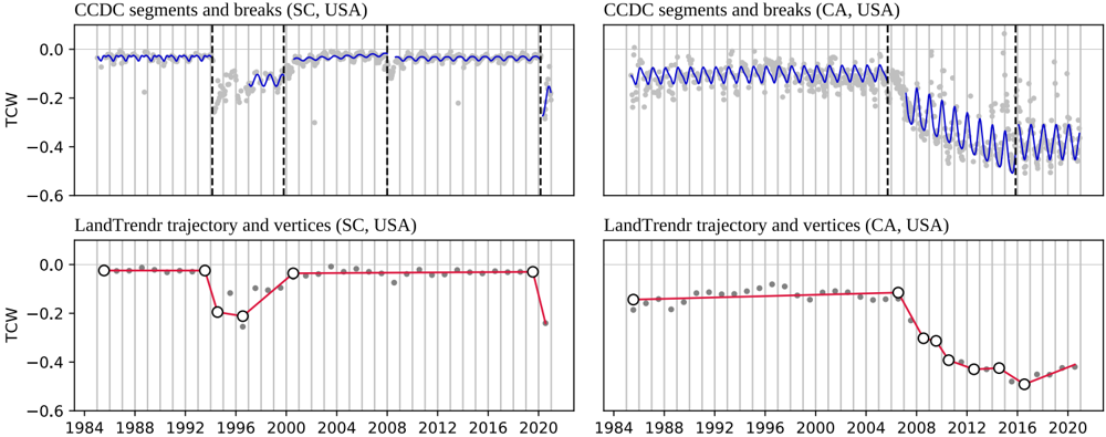
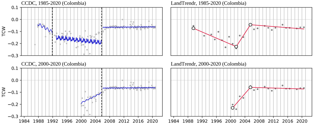
Improved access to remotely sensed imagery and time series algorithms in combination with increased availability of cloud computing resources and platforms such as Google Earth Engine have significantly expanded the community of users processing and analyzing time series of satellite observations. Though individual time series analysis methods and their applications tend to be well-documented, comparisons of different approaches are beneficial to new users faced with the choice of different algorithms and parameterizations. We review two temporal segmentation approaches that have become increasingly prevalent in land cover mapping and monitoring: LandTrendr (Landsat-based detection of Trends in Disturbance and Recovery) and CCDC (Continuous Change Detection and Classification). We examine differences in the way these approaches use the temporal and spectral domains and compare model specifications and outputs. This review highlights previous work and applications, current limitations, ongoing challenges, and opportunities for future integration and comparison of methods and map products, and is expected to benefit both user and developer communities.
Overview
The claims and statistics of this paper haven’t been checked yet.
Free: it reads the open-access text and checks the first 5 claims that cite a source we can check. Create a free account to check every claim.
Integrity signals
Registry
Cites
Statistics
Figures





Verification
Claims the paper makes
The claims and statistics of this paper haven’t been checked yet.
Free: it reads the open-access text and checks the first 5 claims that cite a source we can check. Create a free account to check every claim.
Claims other papers make about this one
Each is checked against this paper’s own text: does it say what the citing paper says it does?
In the citing paper
“We chose to use the CCDC approach because it is (a) well-known and widely used for remote sensing applications (see Pasquarella et al. (2022) for a review) and (b) has already been run globally and surfaced as a dataset, making it one of the few existing examples of a model-as-dataset currently available globally in a cloud-computing environment.”
From AlphaEarth Foundations: An embedding field model for accurate and efficient global mapping from sparse label data (2025) · cites this paper as Pasquarella et al. (2022)
Self-check
Percentages, sums and reported differences re-computed from the paper’s own numbers.
The self-check needs the paper’s full text.
Citations
Cites
No references could be resolved yet.
Research works printed but not linked: 88
- Adams, 2020, Mapping Forest Composition with Landsat Time Series: An Evaluation of Seasonal Composites and Harmonic Regression, Remote Sens., 12, 610, 10.3390/rs12040610 · DOI
- Arévalo, 2020, A Suite of Tools for Continuous Land Change Monitoring in Google Earth Engine, Front. Climate, 2, 10.3389/fclim.2020.576740 · DOI
- Arévalo, 2020, Continuous monitoring of land change activities and post-disturbance dynamics from Landsat time series: A test methodology for REDD+ reporting, Remote Sens. Environ., 238, 111051, 10.1016/j.rse.2019.01.013 · DOI
- Awty-Carroll, 2019, Using Continuous Change Detection and Classification of Landsat Data to Investigate Long-Term Mangrove Dynamics in the Sundarbans Region, Remote Sens., 11, 2833, 10.3390/rs11232833 · DOI
- Awty-Carroll, 2019, An Evaluation and Comparison of Four Dense Time Series Change Detection Methods Using Simulated Data, Remote Sens., 11, 2779, 10.3390/rs11232779 · DOI
- Banskota, 2014, Forest Monitoring Using Landsat Time Series Data: A Review, Can. J. Remote Sens., 40, 362, 10.1080/07038992.2014.987376 · DOI · Paper page
- Berhane, 2020, Land-Cover Changes to Surface-Water Buffers in the Midwestern USA: 25 Years of Landsat Data Analyses (1993–2017), Remote Sens. (Basel), 12, 754, 10.3390/rs12050754 · DOI
- Bright, 2019, Examining post-fire vegetation recovery with Landsat time series analysis in three western North American forest types, Fire Ecol., 15, 1, 10.1186/s42408-018-0021-9 · DOI · Paper page
- Brooks, 2014, On-the-Fly Massively Multitemporal Change Detection Using Statistical Quality Control Charts and Landsat Data, IEEE Trans. Geosci. Remote Sens., 52, 3316, 10.1109/TGRS.2013.2272545 · DOI
- Brown, 2019, Lessons learned implementing an operational continuous United States national land change monitoring capability: The Land Change Monitoring, Assessment, and Project (LCMAP) approach, Remote Sens. Environ.
- Bullock, 2020, Improved change monitoring using an ensemble of time series algorithms, Remote Sens. Environ., 238, 111165, 10.1016/j.rse.2019.04.018 · DOI
- Bullock, 2020, Monitoring tropical forest degradation using spectral unmixing and Landsat time series analysis, Remote Sens. Environ., 238, 110968, 10.1016/j.rse.2018.11.011 · DOI · Paper page
- Chaves, 2020, Recent Applications of Landsat 8/OLI and Sentinel-2/MSI for Land Use and Land Cover Mapping: A Systematic Review, Remote Sens., 12, 3062, 10.3390/rs12183062 · DOI · Paper page
- Chen, 2021, Monitoring temperate forest degradation on Google Earth Engine using Landsat time series analysis, Remote Sens. Environ., 265, 112648, 10.1016/j.rse.2021.112648 · DOI · Paper page
- Cohen, 2017, How Similar Are Forest Disturbance Maps Derived from Different Landsat Time Series Algorithms?, Forests, 8, 98, 10.3390/f8040098 · DOI · Paper page
- Cohen, 2020, Diversity of Algorithm and Spectral Band Inputs Improves Landsat Monitoring of Forest Disturbance, Remote Sens., 12, 1673, 10.3390/rs12101673 · DOI
- Cohen, 2018, A LandTrendr multispectral ensemble for forest disturbance detection, Remote Sens. Environ., 205, 131, 10.1016/j.rse.2017.11.015 · DOI · Paper page
- Coppin, 2004, Review ArticleDigital change detection methods in ecosystem monitoring: a review, Int. J. Remote Sens., 25, 1565, 10.1080/0143116031000101675 · DOI · Paper page
- Dara, 2018, Mapping the timing of cropland abandonment and recultivation in northern Kazakhstan using annual Landsat time series, Remote Sens. Environ., 213, 49, 10.1016/j.rse.2018.05.005 · DOI · Paper page
- de Jong, 2021, Mapping mangrove dynamics and colonization patterns at the Suriname coast using historic satellite data and the LandTrendr algorithm, Int. J. Appl. Earth Obs. Geoinf., 97, 102293
- De Marzo, 2021, Characterizing forest disturbances across the Argentine Dry Chaco based on Landsat time series, Int. J. Appl. Earth Obs. Geoinf., 98, 102310
- Deng, 2020, Continuous subpixel monitoring of urban impervious surface using Landsat time series, Remote Sens. Environ., 238, 110929, 10.1016/j.rse.2018.10.011 · DOI
- Dwyer, 2018, Analysis Ready Data: Enabling Analysis of the Landsat Archive, Remote Sens., 10, 1363, 10.3390/rs10091363 · DOI · Paper page
- Egorov, 2019, Landsat 4, 5 and 7 (1982 to 2017) Analysis Ready Data (ARD) Observation Coverage over the Conterminous United States and Implications for Terrestrial Monitoring, Remote Sens., 11, 447, 10.3390/rs11040447 · DOI
- Frazier, 2015, Boreal Shield forest disturbance and recovery trends using Landsat time series, Remote Sens. Environ., 170, 317, 10.1016/j.rse.2015.09.015 · DOI
- Frazier, 2014, Characterization of aboveground biomass in an unmanaged boreal forest using Landsat temporal segmentation metrics, ISPRS J. Photogramm. Remote Sens., 92, 137, 10.1016/j.isprsjprs.2014.03.003 · DOI
- Fu, 2016, A time series analysis of urbanization induced land use and land cover change and its impact on land surface temperature with Landsat imagery, Remote Sens. Environ., 175, 205, 10.1016/j.rse.2015.12.040 · DOI · Paper page
- Gelabert, 2021, LandTrendr smoothed spectral profiles enhance woody encroachment monitoring, Remote Sens. Environ., 262, 112521, 10.1016/j.rse.2021.112521 · DOI
- Gómez, 2016, Optical remotely sensed time series data for land cover classification: A review, ISPRS J. Photogramm. Remote Sens., 116, 55, 10.1016/j.isprsjprs.2016.03.008 · DOI · Paper page
- Gorelick, 2017, Google Earth Engine: Planetary-scale geospatial analysis for everyone, Remote Sens. Environ., 202, 18, 10.1016/j.rse.2017.06.031 · DOI · Paper page
- Griffiths, 2012, Using annual time-series of Landsat images to assess the effects of forest restitution in post-socialist Romania, Remote Sens. Environ., 118, 199, 10.1016/j.rse.2011.11.006 · doi:10.1016/j.rse.2011.11.006
- Grogan, 2015, Cross-border forest disturbance and the role of natural rubber in mainland Southeast Asia using annual Landsat time series, Remote Sens. Environ., 169, 438, 10.1016/j.rse.2015.03.001 · DOI
- Guan, 2020, Improving land cover change detection and classification with BRDF correction and spatial feature extraction using Landsat time series: a case of urbanization in Tianjin, China, IEEE J. Select. Top. Appl. Earth Observ. Remote Sens., 13, 4166, 10.1109/JSTARS.2020.3007562 · doi:10.1109/jstars.2020.3007562
- Hamunyela, 2020, Implementation of BFASTmonitor Algorithm on Google Earth Engine to Support Large-Area and Sub-Annual Change Monitoring Using Earth Observation Data, Remote Sens., 12, 2953, 10.3390/rs12182953 · DOI
- Healey, 2018, Mapping forest change using stacked generalization: An ensemble approach, Remote Sens. Environ., 204, 717, 10.1016/j.rse.2017.09.029 · DOI · Paper page
- Hemati, 2021, A Systematic Review of Landsat Data for Change Detection Applications: 50 Years of Monitoring the Earth, Remote Sens., 13, 2869, 10.3390/rs13152869 · DOI · Paper page
- Hislop, 2019, A fusion approach to forest disturbance mapping using time series ensemble techniques, Remote Sens. Environ., 221, 188, 10.1016/j.rse.2018.11.025 · DOI
- Hossain, 2019, Segmentation for Object-Based Image Analysis (OBIA): A review of algorithms and challenges from remote sensing perspective, ISPRS J. Photogramm. Remote Sens., 150, 115, 10.1016/j.isprsjprs.2019.02.009 · DOI · Paper page
- Huang, 2010, An automated approach for reconstructing recent forest disturbance history using dense Landsat time series stacks, Remote Sens. Environ., 114, 183, 10.1016/j.rse.2009.08.017 · DOI · Paper page
- Hughes, 2017, Patch-Based Forest Change Detection from Landsat Time Series, Forests, 8, 166, 10.3390/f8050166 · doi:10.3390/f8050166
- Kennedy, 2014, Bringing an ecological view of change to Landsat-based remote sensing, Front. Ecol. Environ., 12, 339, 10.1890/130066 · DOI · Paper page
- Kennedy, 2018, An empirical, integrated forest biomass monitoring system, Environ. Res. Lett., 13, 025004, 10.1088/1748-9326/aa9d9e · doi:10.1088/1748-9326/aa9d9e
- Kennedy, 2010, Detecting trends in forest disturbance and recovery using yearly Landsat time series: 1. LandTrendr — Temporal segmentation algorithms, Remote Sens. Environ., 114, 2897, 10.1016/j.rse.2010.07.008 · DOI · Paper page
- Kennedy, 2012, Spatial and temporal patterns of forest disturbance and regrowth within the area of the Northwest Forest Plan, Remote Sens. Environ., 122, 117, 10.1016/j.rse.2011.09.024 · DOI · Paper page
- Kennedy, 2018, Implementation of the LandTrendr Algorithm on Google Earth Engine, Remote Sens., 10, 691, 10.3390/rs10050691 · DOI · Paper page
- Lister, 2020, Use of Remote Sensing Data to Improve the Efficiency of National Forest Inventories: A Case Study from the United States National Forest Inventory, Forests, 11, 1364, 10.3390/f11121364 · DOI
- Main-Knorn, 2013, Monitoring coniferous forest biomass change using a Landsat trajectory-based approach, Remote Sens. Environ., 139, 277, 10.1016/j.rse.2013.08.010 · DOI
- Meigs, 2015, Spatiotemporal dynamics of recent mountain pine beetle and western spruce budworm outbreaks across the Pacific Northwest Region, USA, For. Ecol. Manage., 339, 71, 10.1016/j.foreco.2014.11.030 · DOI
- Mugiraneza, 2020, Continuous Monitoring of Urban Land Cover Change Trajectories with Landsat Time Series and LandTrendr-Google Earth Engine Cloud Computing, Remote Sens., 12, 2883, 10.3390/rs12182883 · doi:10.3390/rs12182883
- Murillo-Sandoval, 2021, No peace for the forest: Rapid, widespread land changes in the Andes-Amazon region following the Colombian civil war, Glob. Environ. Change, 69, 102283, 10.1016/j.gloenvcha.2021.102283 · DOI
- Nguyen, 2018, A spatial and temporal analysis of forest dynamics using Landsat time-series, Remote Sens. Environ., 217, 461, 10.1016/j.rse.2018.08.028 · DOI
- Pasquarella, 2016, From imagery to ecology: leveraging time series of all available Landsat observations to map and monitor ecosystem state and dynamics, Remote Sens. Ecol. Conserv., 2, 152, 10.1002/rse2.24 · DOI
- Pasquarella, 2018, Improved mapping of forest type using spectral-temporal Landsat features, Remote Sens. Environ., 210, 193, 10.1016/j.rse.2018.02.064 · DOI · Paper page
- Pflugmacher, 2012, Using Landsat-derived disturbance history (1972–2010) to predict current forest structure, Remote Sens. Environ., 122, 146, 10.1016/j.rse.2011.09.025 · DOI · Paper page
- Rathnayake, 2020, Mapping Land Cover Change over a 25-Year Period (1993–2018) in Sri Lanka Using Landsat Time-Series, Land, 9, 27, 10.3390/land9010027 · DOI
- Reilly, 2017, Contemporary patterns of fire extent and severity in forests of the Pacific Northwest, USA (1985–2010), Ecosphere, 8, e01695, 10.1002/ecs2.1695 · DOI · Paper page
- Rodman, 2021, Disturbance detection in Landsat time series is influenced by tree mortality agent and severity, not by prior disturbance, Remote Sens. Environ., 254, 112244, 10.1016/j.rse.2020.112244 · DOI
- Roy, 2016, Characterization of Landsat-7 to Landsat-8 reflective wavelength and normalized difference vegetation index continuity, Remote Sens. Environ., 185, 57, 10.1016/j.rse.2015.12.024 · DOI · Paper page
- Saxena, 2018, Towards a polyalgorithm for land use change detection, ISPRS J. Photogramm. Remote Sens., 144, 217, 10.1016/j.isprsjprs.2018.07.002 · DOI
- Schneibel, 2017, Assessment of spatio-temporal changes of smallholder cultivation patterns in the Angolan Miombo belt using segmentation of Landsat time series, Remote Sens. Environ., 195, 118, 10.1016/j.rse.2017.04.012 · DOI
- Senf, 2015, Characterizing spectral–temporal patterns of defoliator and bark beetle disturbances using Landsat time series, Remote Sens. Environ., 170, 166, 10.1016/j.rse.2015.09.019 · DOI
- Senf, 2021, Mapping the forest disturbance regimes of Europe, Nat. Sustain., 4, 63, 10.1038/s41893-020-00609-y · DOI · Paper page
- Shimizu, 2019, Detecting Forest Changes Using Dense Landsat 8 and Sentinel-1 Time Series Data in Tropical Seasonal Forests, Remote Sens., 11, 1899, 10.3390/rs11161899 · DOI
- Shimizu, 2019, A comprehensive evaluation of disturbance agent classification approaches: Strengths of ensemble classification, multiple indices, spatio-temporal variables, and direct prediction, ISPRS J. Photogramm. Remote Sens., 158, 99, 10.1016/j.isprsjprs.2019.10.004 · DOI
- Sulla-Menashe, 2016, Sources of bias and variability in long-term Landsat time series over Canadian boreal forests, Remote Sens. Environ., 177, 206, 10.1016/j.rse.2016.02.041 · DOI
- Tang, 2019, Mapping forest disturbance across the China-Laos border using annual Landsat time series, Int. J. Remote Sens., 40, 2895, 10.1080/01431161.2018.1533662 · DOI
- Tang, 2019, Near real-time monitoring of tropical forest disturbance: New algorithms and assessment framework, Remote Sens. Environ., 224, 202, 10.1016/j.rse.2019.02.003 · DOI
- Vogeler, 2020, Characterizing over Four Decades of Forest Disturbance in Minnesota, USA, Forests, 11, 362, 10.3390/f11030362 · DOI
- Vogelmann, 2016, Perspectives on monitoring gradual change across the continuity of Landsat sensors using time-series data, Remote Sens. Environ., 185, 258, 10.1016/j.rse.2016.02.060 · DOI · Paper page
- Wilson, 2018, Harmonic regression of Landsat time series for modeling attributes from national forest inventory data, ISPRS J. Photogramm. Remote Sens., 137, 29, 10.1016/j.isprsjprs.2018.01.006 · DOI · Paper page
- Woodcock, 2020, Transitioning from change detection to monitoring with remote sensing: A paradigm shift, Remote Sens. Environ., 238, 111558, 10.1016/j.rse.2019.111558 · DOI
- Wulder, 2012, Opening the archive: How free data has enabled the science and monitoring promise of Landsat, Remote Sens. Environ., 122, 2, 10.1016/j.rse.2012.01.010 · DOI · Paper page
- Wulder, 2016, The global Landsat archive: Status, consolidation, and direction, Remote Sens. Environ., 185, 271, 10.1016/j.rse.2015.11.032 · DOI · Paper page
- Xian, 2021, Implementation of CCDC to produce the LCMAP Collection 1.0 annual land surface change product, Earth Syst. Sci. Data Discuss., 1
- Xiao, 2020, Mapping Annual Land Disturbance and Reclamation in a Surface Coal Mining Region Using Google Earth Engine and the LandTrendr Algorithm: A Case Study of the Shengli Coalfield in Inner Mongolia, China. Remote Sens., 12, 1612, 10.3390/rs12101612 · DOI
- Xu, 2021, Monitoring three-decade dynamics of citrus planting in Southeastern China using dense Landsat records, Int. J. Appl. Earth Obs. Geoinf., 103, 102518
- Xu, 2019, A Scheme for the Long-Term Monitoring of Impervious−Relevant Land Disturbances Using High Frequency Landsat Archives and the Google Earth Engine, Remote Sens., 11, 1891, 10.3390/rs11161891 · DOI
- Yang, 2018, Detecting the dynamics of vegetation disturbance and recovery in surface mining area via Landsat imagery and LandTrendr algorithm, J. Clean. Prod., 178, 353, 10.1016/j.jclepro.2018.01.050 · DOI · Paper page
- Ye, 2021, Developing a new disturbance index for tracking gradual change of forest ecosystems in the hilly red soil region of southern China using dense Landsat time series, Ecol. Inform., 61, 101221, 10.1016/j.ecoinf.2021.101221 · DOI
- Yin, 2018, Mapping agricultural land abandonment from spatial and temporal segmentation of Landsat time series, Remote Sens. Environ., 210, 12, 10.1016/j.rse.2018.02.050 · DOI · Paper page
- Yu, 2021, Quantifying Urban Vegetation Dynamics from a Process Perspective Using Temporally Dense Landsat Imagery, Remote Sens., 13, 3217, 10.3390/rs13163217 · doi:10.3390/rs13163217
- Zhang, 2021, Evaluating the impacts of models, data density and irregularity on reconstructing and forecasting dense Landsat time series, Egypt, J. Remote Sens. Space. Sci., 4, 100023
- Zhu, 2019, Long-Term Monitoring of Cropland Change near Dongting Lake, China, Using the LandTrendr Algorithm with Landsat Imagery, Remote Sens., 11, 1234, 10.3390/rs11101234 · doi:10.3390/rs11101234
- Zhu, 2017, Change detection using Landsat time series: A review of frequencies, preprocessing, algorithms, and applications, ISPRS J. Photogramm. Remote Sens., 130, 370, 10.1016/j.isprsjprs.2017.06.013 · DOI · Paper page
- Zhu, 2016, Optimizing selection of training and auxiliary data for operational land cover classification for the LCMAP initiative, ISPRS J. Photogramm. Remote Sens., 122, 206, 10.1016/j.isprsjprs.2016.11.004 · DOI · Paper page
- Zhu, 2014, Continuous change detection and classification of land cover using all available Landsat data, Remote Sens. Environ., 144, 152, 10.1016/j.rse.2014.01.011 · DOI · Paper page
- Zhu, 2012, Continuous monitoring of forest disturbance using all available Landsat imagery, Remote Sens. Environ., 122, 75, 10.1016/j.rse.2011.10.030 · DOI · Paper page
- Zhu, 2020, Continuous monitoring of land disturbance based on Landsat time series, Remote Sens. Environ., 238, 111116, 10.1016/j.rse.2019.03.009 · DOI · Paper page
Cited by
Venter, Z. S., Barton, D. N., Chakraborty, T., Simensen, T., & Singh, G. (2022) · Remote Sensing · doi:10.3390/rs14164101 · Cited by 380
Brown, C. F., Kazmierski, M. R., Pasquarella, V. J., Rucklidge, W. J., Samsikova, M., Zhang, C., Shelhamer, E., Lahera, E., Wiles, O., Ilyushchenko, S., et al. (2025) · arXiv · doi:10.48550/arxiv.2507.22291 · Cited by 172
Self-citationLópez, J., Qian, Y., Murillo-Sandoval, P. J., Clerici, N., & Eklundh, L. (2024) · Global Ecology and Conservation · doi:10.1016/j.gecco.2024.e03094 · Cited by 9
Metadata
- Authors
- Pasquarella, V. J., Arévalo, P., Bratley, K. H., Bullock, E. L., Gorelick, N., Yang, Z., & Kennedy, R. E.
- Venue
- International Journal of Applied Earth Observation and Geoinformation
- Publisher
- Elsevier BV
- Published
- 2022-06
- Volume
- 110
- Pages
- 102806
- ISSN
- 1569-8432
- Cited by
- 63
- References
- 0
- Language
- en
- Licence
- www.elsevier.com/tdm/userlicense/1.0/ (tdm)
- www.elsevier.com/legal/tdmrep-license (tdm)
- creativecommons.org/licenses/by/4.0/ (vor)
- Funders
- National Aeronautics and Space Administration (80NSSC18K0994)
- U.S. Geological Survey (140G118C0006)
About these checks
Registry, retraction, Cites and statistics results are computed, not judged, with one exception: a printed reference that no index lists is read once by a model before it counts as a citation error. Claims are extracted by a model and kept only when their quote appears verbatim in the text; each cited source is then checked, with a model’s help, for whether it says what the claim relies on. Those verdicts can be wrong — read the claim’s quote and the cited source before relying on one.
Statistics and arithmetic are recomputed, not judged.
Confidence bands are shown only for fields calibrated on our annotated test set. None is calibrated yet, so no band is shown.
What counts as a claim ›How we measure confidence ›How we check this ›
Are you an author, or do you see a problem with this page? Request a review
How to cite
Cite CoChat for the checks on this page, and the paper for its own findings.
- This page
- CoChat. (2026). Citation check: Demystifying LandTrendr and CCDC temporal segmentation. https://app.cochat.ai/papers/10.1016/j.jag.2022.102806
- The paper
- Pasquarella, V. J., Arévalo, P., Bratley, K. H., Bullock, E. L., Gorelick, N., Yang, Z., & Kennedy, R. E. (2022). Demystifying LandTrendr and CCDC temporal segmentation. International Journal of Applied Earth Observation and Geoinformation. https://doi.org/10.1016/j.jag.2022.102806
Data sources
Bibliographic data: Semantic Scholar, OpenAlex, Crossref.
Contains information from the Semantic Scholar Academic Graph Datasets, made available under the ODC Attribution License (ODC-BY 1.0).
Semantic Scholar’s data is described in: Kinney, R., et al. (2023). The Semantic Scholar Open Data Platform. arXiv:2301.10140.
