

The DOI matches its Crossref record; 76 of the 76 references it cites were found in a registry or an index; none of the 14 sources its claims cite is checked for support yet.
Avoiding overstating the strength of forensic evidence: Shrunk likelihood ratios/Bayes factors
Open accessAbstract
When strength of forensic evidence is quantified using sample data and statistical models, a concern may be raised as to whether the output of a model overestimates the strength of evidence. This is particularly the case when the amount of sample data is small, and hence sampling variability is high. This concern is related to concern about precision. This paper describes, explores, and tests three procedures which shrink the value of the likelihood ratio or Bayes factor toward the neutral value of one. The procedures are: (1) a Bayesian procedure with uninformative priors, (2) use of empirical lower and upper bounds (ELUB), and (3) a novel form of regularized logistic regression. As a benchmark, they are compared with linear discriminant analysis, and in some instances with non-regularized logistic regression. The behaviours of the procedures are explored using Monte Carlo simulated data, and tested on real data from comparisons of voice recordings, face images, and glass fragments.
Overview
AI snapshot
Written from the paper’s full text.
TL;DR
This paper describes and tests three shrinkage procedures—Bayesian uninformative Jeffreys priors, empirical lower and upper bounds (ELUB), and regularized logistic regression—for avoiding overstatement of forensic likelihood ratios/Bayes factors, compared with LDA and non-regularized logistic regression. On simulated and real voice, face, and glass data, shrinkage reduced overestimation but often at a cost in Cllr, and the authors prefer regularized logistic regression for casework when data are sparse or distributional assumptions are violated.
Key findings
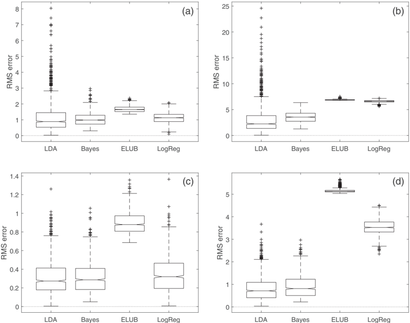
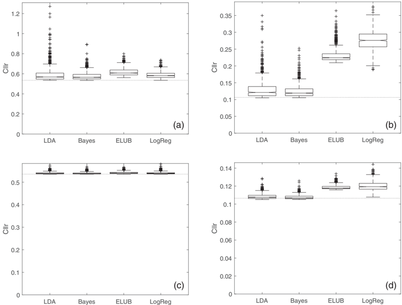
- In Monte Carlo simulations (10 or 100 training samples per category; population means separated by 2 or 4 variance units; 1000 training sets; test set of 1000 per category), the Bayesian procedure outperformed or was not substantially worse than the best procedure across all conditions on RMS error and Cllr; LDA was best when training data were large; ELUB usually performed worst; regularized logistic regression was generally not as good as the Bayesian procedure.
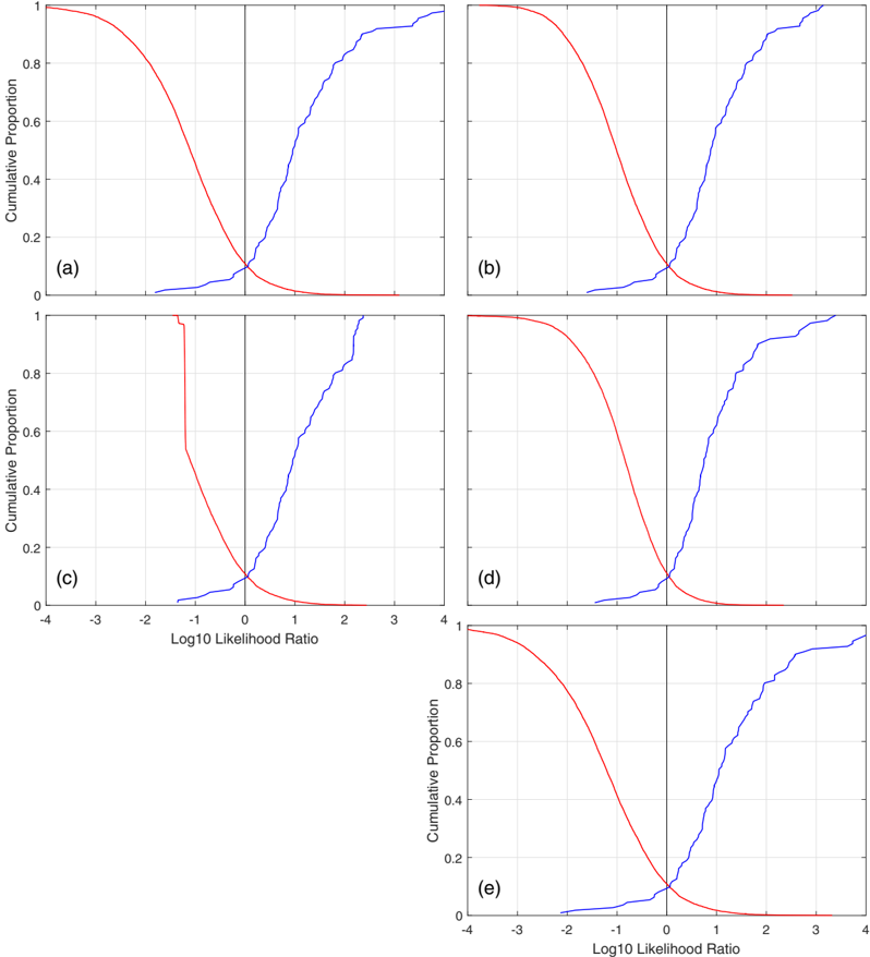
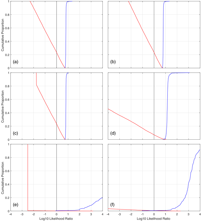
- For real forensic voice comparison, GMM-UBM scores gave Cllr values of 0.410 (LDA), 0.413 (Bayesian), 0.412 (ELUB), 0.430 (regularized logistic regression), and 0.413 (non-regularized logistic regression); i-vector PLDA scores gave 0.357, 0.374, 0.361, 0.290, and 0.261 respectively. In the sisters case, LDA produced extremely large log likelihood ratios (e.g., up to 3×10^40), Bayesian values reached 4876, ELUB gave 5, and regularized logistic regression gave values around 1.6–26.6.
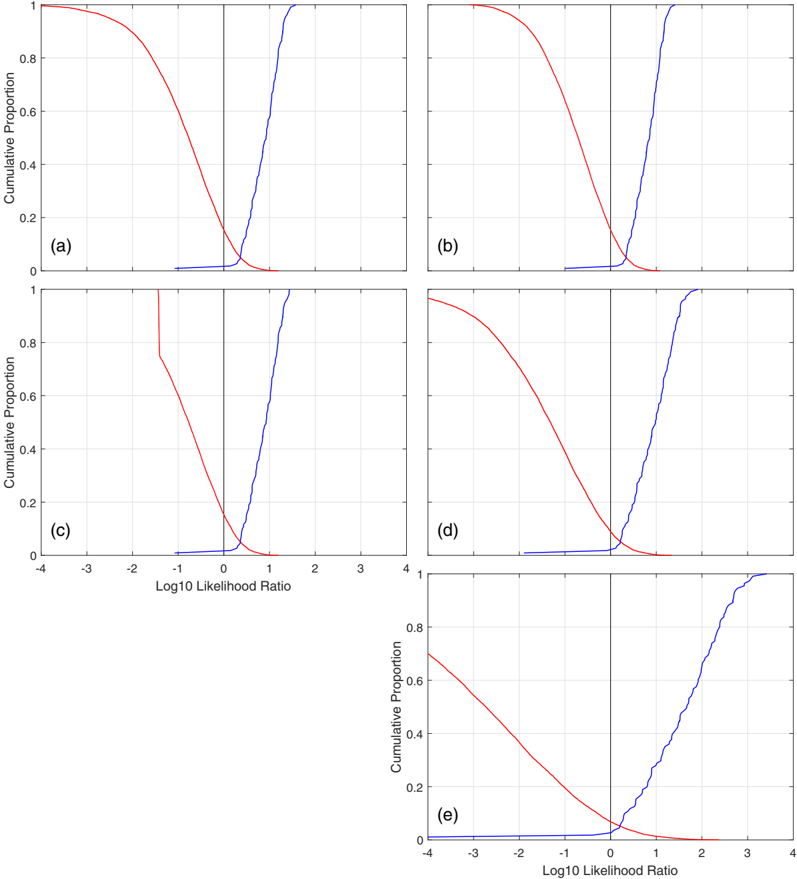
- For face-image comparison, GMM-UBM scores gave Cllr values of 0.220 (LDA), 0.215 (Bayesian), 0.206 (ELUB), 0.181 (regularized logistic regression), and 0.169 (non-regularized logistic regression); MLP scores gave 0.167, 0.159, 0.143, 0.115, and 0.104 respectively. Logistic regression gave the best Cllr, and regularization effected shrinkage with a concomitant decrease in accuracy.
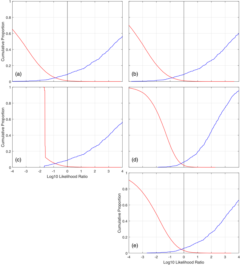
- For glass-fragment comparison, excluding/including very small scores gave Cllr values of 0.391/0.242 (LDA), 0.413/0.236 (Bayesian), 0.389/0.244 (ELUB on LDA), 0.009 (ELUB on tailored model, included only), 0.104/0.111 (regularized logistic regression), and 0.021/0.007 (non-regularized logistic regression). Non-regularized logistic regression performed best; regularized logistic regression was substantially biased in this extreme case.
Methods
- The paper describes and tests three shrinkage procedures—Bayesian model with uninformative Jeffreys reference priors, ELUB applied to LDA output, and a novel regularized logistic regression using a uniform “prior” weighted by κψ pseudodata points—against LDA as a baseline and, on some datasets, non-regularized logistic regression.
- Simulated data were Gaussian same-origin and different-origin score distributions with means of +1 and −1 and common variance 1 (2 variance units), or means separated by 4 variance units; 10 or 100 training samples per category were generated, with 1000 training sets and a test set of 1000 points per category. Performance was assessed using RMS error against reference log likelihood ratios and Cllr.
- Real data came from forensic voice comparison (sisters case with 5 recordings per sister; GMM-UBM and i-vector PLDA scores from 105 speakers for first-stage training and 61 additional speakers for second-stage training/testing, yielding 111 same-speaker and 9720 different-speaker scores), face-image comparison (XM2VTS: 225 faces, 8 images each, 600 same-origin and 40,000 different-origin scores), and glass-fragment comparison (LA-ICP-MS: 979 sources, 659 for first-stage training and 320 for second-stage training/testing, yielding 320 same-origin and 51,040 different-origin scores, of which 41,108 were very small). Cross-validation was used to avoid training and testing on the same data.
Limitations
- Stated: the choice of κψ for regularized logistic regression is essentially arbitrary; κψ = 5 may have induced greater shrinkage than preferred; regularized logistic regression was biased for the glass data because the extreme variance difference affected not only the slope but also the intercept; only an equal-variance Gaussian Bayesian model with Jeffreys reference priors was tested; Cllr does not account for the utility of not overstating strength of evidence, and no such metric was developed.
- Stated: procedures including shrinkage were less accurate and had higher Cllr than their non-shrinkage counterparts; ELUB has a cliff-edge truncation effect; the Bayesian procedure was non-monotonic and produced relatively large Bayes factors that may be difficult to justify given small sample data.
- Evident from the text: the Monte Carlo simulations met the LDA and Bayesian Gaussian equal-variance assumptions, whereas most real datasets violated them; the face-image data used controlled lighting and background and are not reflective of challenging forensic conditions such as CCTV; the sisters case had only 5 recordings per speaker.
Model-written summary. Check it against the paper before relying on it.
Integrity signals
Registry
Cites
Statistics
Figures

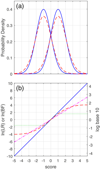
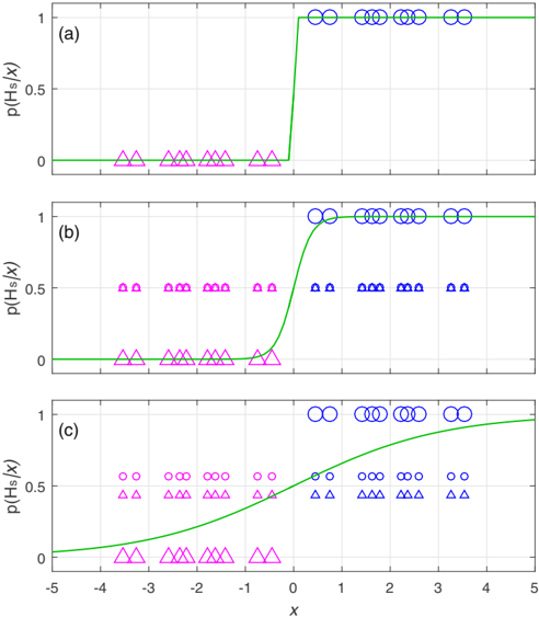
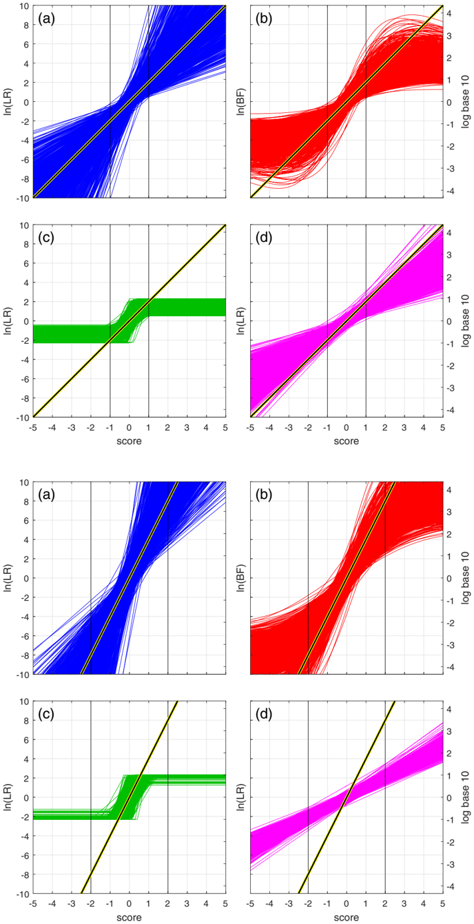
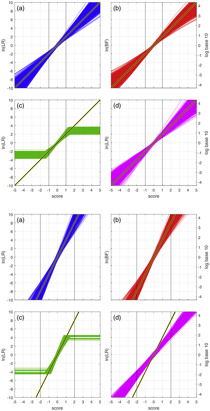
Verification
Claims the paper makes
41 Own result · 27 No basis given · 26 Own interpretation · 11 Sources not found · 4 Own method
A result the paper reports from its own data — it cites no other source for it, so there is none to check. The quote shows it is in the paper.
In the paper
“Non-monotonicity can be observed in some Bayesian functions.”
§ Avoiding overstating the strength of forensic evidence: Shrunk likelihood ratios/Bayes factors > 4. Exploration of the behaviour of the four procedures using simulated data
plain- Asserted: passes — The authors put it forward as true.
- Checkable: passes — It can be checked against evidence.
- Load-bearing: unclear — It is unclear whether the paper’s conclusions depend on it.
- Based: passes — The paper gives a reason why it holds.
A result the paper reports from its own data — it cites no other source for it, so there is none to check. The quote shows it is in the paper.
In the paper
“The LDA procedure resulted in extremely large magnitude log likelihood ratio values, that would be difficult to justify give any realistic amount of training data, let alone 5 recordings per speaker.”
§ Avoiding overstating the strength of forensic evidence: Shrunk likelihood ratios/Bayes factors > 5.1. Forensic comparison of voice recordings: sisters case
hedgeddirectSingle case- Asserted: passes — The authors put it forward as true.
- Checkable: passes — It can be checked against evidence.
- Load-bearing: passes — The paper’s conclusions depend on it.
- Based: passes — The paper gives a reason why it holds.
A result the paper reports from its own data — it cites no other source for it, so there is none to check. The quote shows it is in the paper.
In the paper
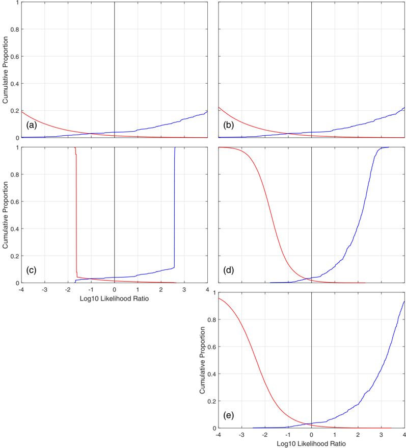
“Both these procedures applied to both sets of scores also produced some very large magnitude log likelihood ratio values (beyond the -4 to +4 range plotted on the Tippett plots) which would be difficult to justify given the amount of training data.”
§ Avoiding overstating the strength of forensic evidence: Shrunk likelihood ratios/Bayes factors > 5.3. Forensic comparison of face images
hedged- Asserted: passes — The authors put it forward as true.
- Checkable: passes — It can be checked against evidence.
- Load-bearing: passes — The paper’s conclusions depend on it.
- Based: passes — The paper gives a reason why it holds.
A result the paper reports from its own data — it cites no other source for it, so there is none to check. The quote shows it is in the paper.
In the paper
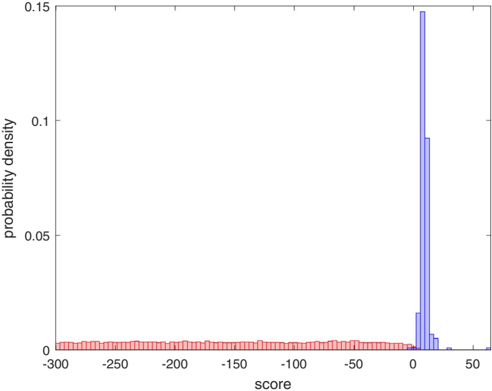
“41,108 of the differentorigin scores had values which were smaller than the smallest encodable value in the software used to calculate them”
§ Avoiding overstating the strength of forensic evidence: Shrunk likelihood ratios/Bayes factors > 5.4. Forensic comparison of glass fragments
plain- Asserted: passes — The authors put it forward as true.
- Checkable: passes — It can be checked against evidence.
- Load-bearing: passes — The paper’s conclusions depend on it.
- Based: passes — The paper gives a reason why it holds.
A result the paper reports from its own data — it cites no other source for it, so there is none to check. The quote shows it is in the paper.
In the paper
“The ELUB procedure usually performed the worst on these metrics.”
§ Avoiding overstating the strength of forensic evidence: Shrunk likelihood ratios/Bayes factors > 4. Exploration of the behaviour of the four procedures using simulated data
plain- Asserted: passes — The authors put it forward as true.
- Checkable: passes — It can be checked against evidence.
- Load-bearing: passes — The paper’s conclusions depend on it.
- Based: passes — The paper gives a reason why it holds.
A result the paper reports from its own data — it cites no other source for it, so there is none to check. The quote shows it is in the paper.
In the paper
“Given a larger amount of training data (Figs. 5 and 6), the relative effect of shrinkage is less.”
§ Avoiding overstating the strength of forensic evidence: Shrunk likelihood ratios/Bayes factors > 4. Exploration of the behaviour of the four procedures using simulated data
plaincorrelational- Asserted: passes — The authors put it forward as true.
- Checkable: passes — It can be checked against evidence.
- Load-bearing: unclear — It is unclear whether the paper’s conclusions depend on it.
- Based: passes — The paper gives a reason why it holds.
The paper states this without a source or data behind it here, so there is nothing to check it against. The quote shows it is in the paper.
In the paper
“ELUB gave very conservative results.”
§ Avoiding overstating the strength of forensic evidence: Shrunk likelihood ratios/Bayes factors > 5.1. Forensic comparison of voice recordings: sisters case
plain- Asserted: passes — The authors put it forward as true.
- Checkable: passes — It can be checked against evidence.
- Load-bearing: passes — The paper’s conclusions depend on it.
- Based: passes — The paper gives a reason why it holds.
A result the paper reports from its own data — it cites no other source for it, so there is none to check. The quote shows it is in the paper.
In the paper
“These scores exhibit an extreme case of non-equal variance.”
§ Avoiding overstating the strength of forensic evidence: Shrunk likelihood ratios/Bayes factors > 5.4. Forensic comparison of glass fragments
plain- Asserted: passes — The authors put it forward as true.
- Checkable: passes — It can be checked against evidence.
- Load-bearing: passes — The paper’s conclusions depend on it.
- Based: passes — The paper gives a reason why it holds.
A result the paper reports from its own data — it cites no other source for it, so there is none to check. The quote shows it is in the paper.
In the paper
“Non-regularized logistic regression gave by far the best performance in terms of C llr”
§ Avoiding overstating the strength of forensic evidence: Shrunk likelihood ratios/Bayes factors > 5.4. Forensic comparison of glass fragments
plaincorrelational- Asserted: passes — The authors put it forward as true.
- Checkable: passes — It can be checked against evidence.
- Load-bearing: unclear — It is unclear whether the paper’s conclusions depend on it.
- Based: passes — The paper gives a reason why it holds.
A result the paper reports from its own data — it cites no other source for it, so there is none to check. The quote shows it is in the paper.
In the paper
“The LDA functions (Fig. 3a) have a substantial variation in log likelihood ratio values (vertical spread)”
§ Avoiding overstating the strength of forensic evidence: Shrunk likelihood ratios/Bayes factors > 4. Exploration of the behaviour of the four procedures using simulated data
plain- Asserted: passes — The authors put it forward as true.
- Checkable: passes — It can be checked against evidence.
- Load-bearing: passes — The paper’s conclusions depend on it.
- Based: passes — The paper gives a reason why it holds.
- It may state two separate claims as one. 38
- The quote only partly states this claim. 3
- Probably not a substantial claim. 15
A result the paper reports from its own data — it cites no other source for it, so there is none to check. The quote shows it is in the paper.
In the paper
“Across all condition, and for both metrics, the Bayesian procedure outperformed the other procedures or was not substantially worse than the best performing system for a condition.”
§ Avoiding overstating the strength of forensic evidence: Shrunk likelihood ratios/Bayes factors > 4. Exploration of the behaviour of the four procedures using simulated data
plain- Asserted: passes — The authors put it forward as true.
- Checkable: passes — It can be checked against evidence.
- Load-bearing: passes — The paper’s conclusions depend on it.
- Based: passes — The paper gives a reason why it holds.
It may state two separate claims as one.
A result the paper reports from its own data — it cites no other source for it, so there is none to check. The quote shows it is in the paper.
In the paper
“Performance was very slightly better than that of the i-vector system alone: C llr was 0.286 and 0.241 for the regularized and non-regularized procedures respectively.”
§ Avoiding overstating the strength of forensic evidence: Shrunk likelihood ratios/Bayes factors > 5.2. Forensic comparison of voice recordings: scores from GMM-UBM and ivector PLDA systems
plain- Asserted: passes — The authors put it forward as true.
- Checkable: passes — It can be checked against evidence.
- Load-bearing: unclear — It is unclear whether the paper’s conclusions depend on it.
- Based: passes — The paper gives a reason why it holds.
It may state two separate claims as one.
A result the paper reports from its own data — it cites no other source for it, so there is none to check. The quote shows it is in the paper.
In the paper
“Both deviate from the assumptions of Gaussian distributions with equal variance.”
§ Avoiding overstating the strength of forensic evidence: Shrunk likelihood ratios/Bayes factors > 5.3. Forensic comparison of face images
plain- Asserted: passes — The authors put it forward as true.
- Checkable: passes — It can be checked against evidence.
- Load-bearing: passes — The paper’s conclusions depend on it.
- Based: passes — The paper gives a reason why it holds.
It may state two separate claims as one.
A result the paper reports from its own data — it cites no other source for it, so there is none to check. The quote shows it is in the paper.
In the paper
“The Bayesian functions (Fig. 3b) have a substantial variation in log Bayes factor values (vertical spread), but on average less than the variation of log likelihood ratio values for the LDA functions.”
§ Avoiding overstating the strength of forensic evidence: Shrunk likelihood ratios/Bayes factors > 4. Exploration of the behaviour of the four procedures using simulated data
plain- Asserted: passes — The authors put it forward as true.
- Checkable: passes — It can be checked against evidence.
- Load-bearing: passes — The paper’s conclusions depend on it.
- Based: passes — The paper gives a reason why it holds.
It may state two separate claims as one.
A result the paper reports from its own data — it cites no other source for it, so there is none to check. The quote shows it is in the paper.
In the paper
“When the amount of training data was large, LDA outperformed the other procedures on both metrics or was not substantially worse than the best performing system for a condition.”
§ Avoiding overstating the strength of forensic evidence: Shrunk likelihood ratios/Bayes factors > 4. Exploration of the behaviour of the four procedures using simulated data
plain- Asserted: passes — The authors put it forward as true.
- Checkable: passes — It can be checked against evidence.
- Load-bearing: unclear — It is unclear whether the paper’s conclusions depend on it.
- Based: passes — The paper gives a reason why it holds.
It may state two separate claims as one.
A result the paper reports from its own data — it cites no other source for it, so there is none to check. The quote shows it is in the paper.
In the paper
“The regularized logistic regression functions exhibit shrinkage, they are almost always closer to 0 than the reference value functions.”
§ Avoiding overstating the strength of forensic evidence: Shrunk likelihood ratios/Bayes factors > 4. Exploration of the behaviour of the four procedures using simulated data
plaincorrelational- Asserted: passes — The authors put it forward as true.
- Checkable: passes — It can be checked against evidence.
- Load-bearing: unclear — It is unclear whether the paper’s conclusions depend on it.
- Based: passes — The paper gives a reason why it holds.
It may state two separate claims as one.
A result the paper reports from its own data — it cites no other source for it, so there is none to check. The quote shows it is in the paper.
In the paper
“Regularized logistic regression resulted in likelihood ratio values around the same size as those from ELUB, but which could be up to several times larger or several times smaller.”
§ Avoiding overstating the strength of forensic evidence: Shrunk likelihood ratios/Bayes factors > 5.1. Forensic comparison of voice recordings: sisters case
hedgedcorrelationalSingle case- Asserted: passes — The authors put it forward as true.
- Checkable: passes — It can be checked against evidence.
- Load-bearing: unclear — It is unclear whether the paper’s conclusions depend on it.
- Based: passes — The paper gives a reason why it holds.
It may state two separate claims as one.
The paper states this without a source or data behind it here, so there is nothing to check it against. The quote shows it is in the paper.
In the paper
“The Bayesian functions are sigmoidal and the rate at which they deviate from 0 is close to that of the reference function for low reference values, but decreases as the magnitude of the reference values increase.”
§ Avoiding overstating the strength of forensic evidence: Shrunk likelihood ratios/Bayes factors > 4. Exploration of the behaviour of the four procedures using simulated data
plaindirect- Asserted: passes — The authors put it forward as true.
- Checkable: passes — It can be checked against evidence.
- Load-bearing: unclear — It is unclear whether the paper’s conclusions depend on it.
- Based: passes — The paper gives a reason why it holds.
It may state two separate claims as one.
A result the paper reports from its own data — it cites no other source for it, so there is none to check. The quote shows it is in the paper.
In the paper
“Bias was much smaller for the logistic regression results, and the range of log likelihood ratio values produced were more reasonable.”
§ Avoiding overstating the strength of forensic evidence: Shrunk likelihood ratios/Bayes factors > 5.3. Forensic comparison of face images
plaincorrelational- Asserted: passes — The authors put it forward as true.
- Checkable: passes — It can be checked against evidence.
- Load-bearing: passes — The paper’s conclusions depend on it.
- Based: passes — The paper gives a reason why it holds.
It may state two separate claims as one.
A result the paper reports from its own data — it cites no other source for it, so there is none to check. The quote shows it is in the paper.
In the paper
“Regularizing the logistic regression model effected substantial shrinkage.”
§ Avoiding overstating the strength of forensic evidence: Shrunk likelihood ratios/Bayes factors > 5.2. Forensic comparison of voice recordings: scores from GMM-UBM and ivector PLDA systems
plaindirect- Asserted: passes — The authors put it forward as true.
- Checkable: passes — It can be checked against evidence.
- Load-bearing: passes — The paper’s conclusions depend on it.
- Based: passes — The paper gives a reason why it holds.
The quote only partly states this claim.
A result the paper reports from its own data — it cites no other source for it, so there is none to check. The quote shows it is in the paper.
In the paper
“When the separation between the categories is greater and the amount of data is larger, the ELUB bounds are further from 0 and the slopes of the regularized logistic regression functions increase”
§ Avoiding overstating the strength of forensic evidence: Shrunk likelihood ratios/Bayes factors > 4. Exploration of the behaviour of the four procedures using simulated data
plaindirect- Asserted: passes — The authors put it forward as true.
- Checkable: passes — It can be checked against evidence.
- Load-bearing: unclear — It is unclear whether the paper’s conclusions depend on it.
- Based: passes — The paper gives a reason why it holds.
It may state two separate claims as one.
A result the paper reports from its own data — it cites no other source for it, so there is none to check. The quote shows it is in the paper.
In the paper
“Logistic regression gave the best results in terms of C llr , and regularizing the logistic regression model effected shrinkage, with a concomitant decrease in accuracy (an increase in C llr ).”
§ Avoiding overstating the strength of forensic evidence: Shrunk likelihood ratios/Bayes factors > 5.3. Forensic comparison of face images
plaindirect- Asserted: passes — The authors put it forward as true.
- Checkable: passes — It can be checked against evidence.
- Load-bearing: passes — The paper’s conclusions depend on it.
- Based: passes — The paper gives a reason why it holds.
It may state two separate claims as one.
A result the paper reports from its own data — it cites no other source for it, so there is none to check. The quote shows it is in the paper.
In the paper
“All procedures give more precise results, and the procedures involving shrinkage also give more accurate results.”
§ Avoiding overstating the strength of forensic evidence: Shrunk likelihood ratios/Bayes factors > 4. Exploration of the behaviour of the four procedures using simulated data
plaindirect- Asserted: passes — The authors put it forward as true.
- Checkable: passes — It can be checked against evidence.
- Load-bearing: passes — The paper’s conclusions depend on it.
- Based: passes — The paper gives a reason why it holds.
It may state two separate claims as one.
The paper states this without a source or data behind it here, so there is nothing to check it against. The quote shows it is in the paper.
In the paper
“With such a small amount of data, the posterior predictive distributions are substantially broader and flatter than the sample distributions.”
§ Avoiding overstating the strength of forensic evidence: Shrunk likelihood ratios/Bayes factors > 1. Introduction
plaindirectn = 10- Asserted: passes — The authors put it forward as true.
- Checkable: passes — It can be checked against evidence.
- Load-bearing: passes — The paper’s conclusions depend on it.
- Based: passes — The paper gives a reason why it holds.
The quote only partly states this claim.
- The authors state this as an assumption: The sample data used in the Bayesian model are from a Gaussian distribution with unknown mean and variance.
A result the paper reports from its own data — it cites no other source for it, so there is none to check. The quote shows it is in the paper.
In the paper
“The regularized logistic regression functions (Fig. 3d) have substantial variation in log likelihood ratio values (vertical spread), but substantially less than that for the LDA functions.”
§ Avoiding overstating the strength of forensic evidence: Shrunk likelihood ratios/Bayes factors > 4. Exploration of the behaviour of the four procedures using simulated data
plaincorrelational- Asserted: passes — The authors put it forward as true.
- Checkable: passes — It can be checked against evidence.
- Load-bearing: passes — The paper’s conclusions depend on it.
- Based: passes — The paper gives a reason why it holds.
It may state two separate claims as one.
The paper states this without a source or data behind it here, so there is nothing to check it against. The quote shows it is in the paper.
In the paper
“The calculation of different-speaker scores reuses each recording multiple times, and thus the score values are not statistically independent.”
§ Avoiding overstating the strength of forensic evidence: Shrunk likelihood ratios/Bayes factors > 3.4. Regularized logistic regression
plaindirect- Asserted: passes — The authors put it forward as true.
- Checkable: passes — It can be checked against evidence.
- Load-bearing: passes — The paper’s conclusions depend on it.
- Based: passes — The paper gives a reason why it holds.
It may state two separate claims as one.
A result the paper reports from its own data — it cites no other source for it, so there is none to check. The quote shows it is in the paper.
In the paper
“The Bayesian procedure resulted in smaller log Bayes factor values, 17 but still reaching values that may be difficult to justify given the small amount of training data.”
§ Avoiding overstating the strength of forensic evidence: Shrunk likelihood ratios/Bayes factors > 5.1. Forensic comparison of voice recordings: sisters case
hedgeddirectSingle case- Asserted: passes — The authors put it forward as true.
- Checkable: passes — It can be checked against evidence.
- Load-bearing: passes — The paper’s conclusions depend on it.
- Based: passes — The paper gives a reason why it holds.
It may state two separate claims as one.
A result the paper reports from its own data — it cites no other source for it, so there is none to check. The quote shows it is in the paper.
In the paper
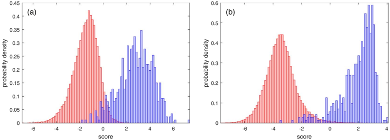
“The assumption of equal variance is clearly violated, and the same-origin scores are skewed, the skewness being more pronounced for the MLP system.”
§ Avoiding overstating the strength of forensic evidence: Shrunk likelihood ratios/Bayes factors > 5.3. Forensic comparison of face images
boostedcorrelational- Asserted: passes — The authors put it forward as true.
- Checkable: passes — It can be checked against evidence.
- Load-bearing: passes — The paper’s conclusions depend on it.
- Based: passes — The paper gives a reason why it holds.
It may state two separate claims as one.
A result the paper reports from its own data — it cites no other source for it, so there is none to check. The quote shows it is in the paper.
In the paper
“For the scores from the GMM-UBM system, the assumptions of normality and equal variance appear to be met.”
§ Avoiding overstating the strength of forensic evidence: Shrunk likelihood ratios/Bayes factors > 5.2. Forensic comparison of voice recordings: scores from GMM-UBM and ivector PLDA systems
hedged- Asserted: passes — The authors put it forward as true.
- Checkable: passes — It can be checked against evidence.
- Load-bearing: unclear — It is unclear whether the paper’s conclusions depend on it.
- Based: passes — The paper gives a reason why it holds.
It may state two separate claims as one.
A result the paper reports from its own data — it cites no other source for it, so there is none to check. The quote shows it is in the paper.
In the paper
“regularization effected substantial shrinkage with a concomitant loss in accuracy (although still a substantially lower C llr than the other procedures).”
§ Avoiding overstating the strength of forensic evidence: Shrunk likelihood ratios/Bayes factors > 5.4. Forensic comparison of glass fragments
plaindirect- Asserted: passes — The authors put it forward as true.
- Checkable: passes — It can be checked against evidence.
- Load-bearing: passes — The paper’s conclusions depend on it.
- Based: passes — The paper gives a reason why it holds.
It may state two separate claims as one.
The paper states this without a source or data behind it here, so there is nothing to check it against. The quote shows it is in the paper.
In the paper
“The ELUB functions (Fig. 3c) follow the LDA functions for low magnitude reference values (by design), and are then suddenly truncated.”
§ Avoiding overstating the strength of forensic evidence: Shrunk likelihood ratios/Bayes factors > 4. Exploration of the behaviour of the four procedures using simulated data
plaincorrelational- Asserted: passes — The authors put it forward as true.
- Checkable: passes — It can be checked against evidence.
- Load-bearing: unclear — It is unclear whether the paper’s conclusions depend on it.
- Based: passes — The paper gives a reason why it holds.
It may state two separate claims as one.
A result the paper reports from its own data — it cites no other source for it, so there is none to check. The quote shows it is in the paper.
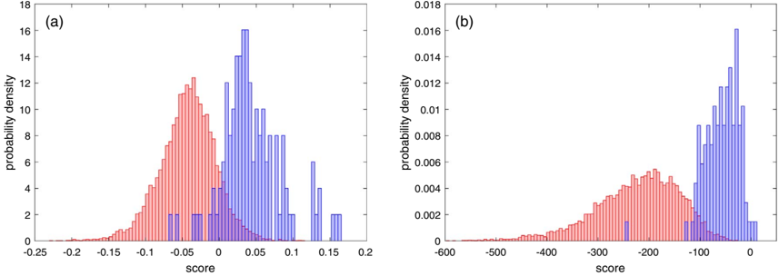
In the paper
“For the scores from the i-vector PLDA system, the different-speaker scores have a slight skew, and the assumption of equal variance is clearly violated.”
§ Avoiding overstating the strength of forensic evidence: Shrunk likelihood ratios/Bayes factors > 5.2. Forensic comparison of voice recordings: scores from GMM-UBM and ivector PLDA systems
boosted- Asserted: passes — The authors put it forward as true.
- Checkable: passes — It can be checked against evidence.
- Load-bearing: passes — The paper’s conclusions depend on it.
- Based: passes — The paper gives a reason why it holds.
It may state two separate claims as one.
The paper states this without a source or data behind it here, so there is nothing to check it against. The quote shows it is in the paper.
In the paper
“Unlike the Bayesian and ELUB functions, the regularized logistic regression functions are linear.”
§ Avoiding overstating the strength of forensic evidence: Shrunk likelihood ratios/Bayes factors > 4. Exploration of the behaviour of the four procedures using simulated data
plain- Asserted: passes — The authors put it forward as true.
- Checkable: passes — It can be checked against evidence.
- Load-bearing: fails — The paper’s conclusions may not depend on it.
- Based: passes — The paper gives a reason why it holds.
Probably not a substantial claim. The paper’s conclusions may not depend on it.
A result the paper reports from its own data — it cites no other source for it, so there is none to check. The quote shows it is in the paper.
In the paper
“The Bayesian procedure and regularized logistic regression effected shrinkage, which was greatest for the latter.”
§ Avoiding overstating the strength of forensic evidence: Shrunk likelihood ratios/Bayes factors > 5.2. Forensic comparison of voice recordings: scores from GMM-UBM and ivector PLDA systems
plaindirect- Asserted: passes — The authors put it forward as true.
- Checkable: passes — It can be checked against evidence.
- Load-bearing: unclear — It is unclear whether the paper’s conclusions depend on it.
- Based: passes — The paper gives a reason why it holds.
It may state two separate claims as one.
The paper states this without a source or data behind it here, so there is nothing to check it against. The quote shows it is in the paper.
In the paper
“LDA and the Bayesian procedure depend on assumptions of Gaussian distributions with equal variance and, as expected, performed poorly on these data.”
§ Avoiding overstating the strength of forensic evidence: Shrunk likelihood ratios/Bayes factors > 5.4. Forensic comparison of glass fragments
plaindirect- Asserted: passes — The authors put it forward as true.
- Checkable: passes — It can be checked against evidence.
- Load-bearing: passes — The paper’s conclusions depend on it.
- Based: passes — The paper gives a reason why it holds.
It may state two separate claims as one.
- Rests on an assumption: LDA and Bayesian procedures depend on assumptions of Gaussian distributions with equal variance.
A result the paper reports from its own data — it cites no other source for it, so there is none to check. The quote shows it is in the paper.
In the paper
“Shrinkage came at the cost of a decrease in accuracy (an increase in C llr ).”
§ Avoiding overstating the strength of forensic evidence: Shrunk likelihood ratios/Bayes factors > 5.2. Forensic comparison of voice recordings: scores from GMM-UBM and ivector PLDA systems
plaindirect- Asserted: passes — The authors put it forward as true.
- Checkable: passes — It can be checked against evidence.
- Load-bearing: passes — The paper’s conclusions depend on it.
- Based: passes — The paper gives a reason why it holds.
The quote only partly states this claim.
A conclusion the paper draws from its own results — it cites no other source for it, so there is none to check. The quote shows it is in the paper.
In the paper
“x d i and x s j with low weights will have p d i and p s j values close to 0.5, whereas x d i and x s j with high weights will have p d i and p s j values close to 0 and 1 respectively.”
§ Avoiding overstating the strength of forensic evidence: Shrunk likelihood ratios/Bayes factors > 3.4. Regularized logistic regression
plaincorrelational- Asserted: passes — The authors put it forward as true.
- Checkable: passes — It can be checked against evidence.
- Load-bearing: unclear — It is unclear whether the paper’s conclusions depend on it.
- Based: passes — The paper gives a reason why it holds.
It may state two separate claims as one.
The paper states this without a source or data behind it here, so there is nothing to check it against. The quote shows it is in the paper.
In the paper
“Given a large amount of sample data and assuming models appropriate for fitting the population distributions, the modelled sample distributions will be reasonable approximations of the population distributions, and a calculated likelihood ratio value will be a reasonable estimate of the true but unknown likelihood ratio value.”
§ Avoiding overstating the strength of forensic evidence: Shrunk likelihood ratios/Bayes factors > 1. Introduction
plainconditional- Asserted: passes — The authors put it forward as true.
- Checkable: passes — It can be checked against evidence.
- Load-bearing: passes — The paper’s conclusions depend on it.
- Based: fails — The paper may give no reason why it holds.
Probably not a substantial claim. The paper may give no reason why it holds. It may state two separate claims as one.
- The authors state this as an assumption: The models fitted to the population distributions are appropriate.
A conclusion the paper draws from its own results — it cites no other source for it, so there is none to check. The quote shows it is in the paper.
In the paper
“Based on the reported results using these metrics, the Bayesian procedure would be preferred.”
§ Avoiding overstating the strength of forensic evidence: Shrunk likelihood ratios/Bayes factors > 4. Exploration of the behaviour of the four procedures using simulated data
hedged- Asserted: passes — The authors put it forward as true.
- Checkable: passes — It can be checked against evidence.
- Load-bearing: passes — The paper’s conclusions depend on it.
- Based: passes — The paper gives a reason why it holds.
Probably not a substantial claim.
A conclusion the paper draws from its own results — it cites no other source for it, so there is none to check. The quote shows it is in the paper.
In the paper
“Both procedures exhibit a property known as shrinkage.”
§ Avoiding overstating the strength of forensic evidence: Shrunk likelihood ratios/Bayes factors > 1. Introduction
plaincorrelational- Asserted: passes — The authors put it forward as true.
- Checkable: passes — It can be checked against evidence.
- Load-bearing: passes — The paper’s conclusions depend on it.
- Based: passes — The paper gives a reason why it holds.
It may state two separate claims as one.
A conclusion the paper draws from its own results — it cites no other source for it, so there is none to check. The quote shows it is in the paper.
In the paper
“Whatever the data, the slope fitted using regularization will be shallower than for a model not including regularization, but, apart from in circumstances involving complete or near complete separation, the difference in slope will be slight if the regularization weight is small.”
§ Avoiding overstating the strength of forensic evidence: Shrunk likelihood ratios/Bayes factors > 3.4. Regularized logistic regression
plaindirect- Asserted: passes — The authors put it forward as true.
- Checkable: passes — It can be checked against evidence.
- Load-bearing: unclear — It is unclear whether the paper’s conclusions depend on it.
- Based: unclear — It is unclear why the paper says it holds.
It may state two separate claims as one.
A conclusion the paper draws from its own results — it cites no other source for it, so there is none to check. The quote shows it is in the paper.
In the paper
“The model is linear in the logistic space (i.e., the logged odds space), and the fitted intercept and slope values in the logistic space can therefore be used to convert a score x to a log likelihood ratio ln(Λ LogReg ) as in Eq. ( 8).”
§ Avoiding overstating the strength of forensic evidence: Shrunk likelihood ratios/Bayes factors > 3.4. Regularized logistic regression
plaindirect- Asserted: passes — The authors put it forward as true.
- Checkable: passes — It can be checked against evidence.
- Load-bearing: passes — The paper’s conclusions depend on it.
- Based: passes — The paper gives a reason why it holds.
It may state two separate claims as one.
A conclusion the paper draws from its own results — it cites no other source for it, so there is none to check. The quote shows it is in the paper.
In the paper
“Two Bayesians starting with different priors will arrive at different posterior predictive distributions when the amount of sample data is small, but their posterior predictive distributions will converge on the sample distribution as the amount of sample data increases.”
§ Avoiding overstating the strength of forensic evidence: Shrunk likelihood ratios/Bayes factors > 1. Introduction
plaindirect- Asserted: passes — The authors put it forward as true.
- Checkable: passes — It can be checked against evidence.
- Load-bearing: unclear — It is unclear whether the paper’s conclusions depend on it.
- Based: passes — The paper gives a reason why it holds.
It may state two separate claims as one.
In the paper
“Use of the same variance for both Gaussians ensures that the score to likelihood ratio conversion function is linear, and hence monotonic, [12,18 §6.5.2.1, 28,32].”
§ Avoiding overstating the strength of forensic evidence: Shrunk likelihood ratios/Bayes factors > 3.1. Linear discriminant analysis (LDA)
What the sources say
- Not matchedcites [12,18 §6.5.2.1, 28,32]
Couldn’t be matched to a paper in Crossref, so it can’t be checked.
plaindirect- Asserted: passes — The authors put it forward as true.
- Checkable: passes — It can be checked against evidence.
- Load-bearing: unclear — It is unclear whether the paper’s conclusions depend on it.
- Based: passes — The paper gives a reason why it holds.
It may state two separate claims as one.
- The authors state this as an assumption: The data used for LDA have Gaussian distributions with equal variance.
- Not matched
In the paper
“Adding the copies removes the complete separation in the training data and the algorithm converges on a non-infinite slope.”
§ Avoiding overstating the strength of forensic evidence: Shrunk likelihood ratios/Bayes factors > 3.4. Regularized logistic regression
What the sources say
- Not matchedcites [44]
Couldn’t be matched to a paper in Crossref, so it can’t be checked.
plaindirect- Asserted: passes — The authors put it forward as true.
- Checkable: passes — It can be checked against evidence.
- Load-bearing: passes — The paper’s conclusions depend on it.
- Based: passes — The paper gives a reason why it holds.
It may state two separate claims as one.
- Not matched
A conclusion the paper draws from its own results — it cites no other source for it, so there is none to check. The quote shows it is in the paper.
In the paper
“The regularized logistic regression procedure could have advantages when these assumptions are violated.”
§ Avoiding overstating the strength of forensic evidence: Shrunk likelihood ratios/Bayes factors > 4. Exploration of the behaviour of the four procedures using simulated data
hedgedconditional- Asserted: passes — The authors put it forward as true.
- Checkable: passes — It can be checked against evidence.
- Load-bearing: fails — The paper’s conclusions may not depend on it.
- Based: passes — The paper gives a reason why it holds.
Probably not a substantial claim. The paper’s conclusions may not depend on it.
In the paper
“Logistic regression, however, is not dependent on these assumptions, and hence is more robust to violations of these assumptions than is LDA, [37] §4.4.5.”
§ Avoiding overstating the strength of forensic evidence: Shrunk likelihood ratios/Bayes factors > 3.4. Regularized logistic regression
What the sources say
- Not matchedcites [37] §4.4.5
Couldn’t be matched to a paper in Crossref, so it can’t be checked.
plaindirect- Asserted: passes — The authors put it forward as true.
- Checkable: passes — It can be checked against evidence.
- Load-bearing: passes — The paper’s conclusions depend on it.
- Based: passes — The paper gives a reason why it holds.
It may state two separate claims as one.
- Not matched
A conclusion the paper draws from its own results — it cites no other source for it, so there is none to check. The quote shows it is in the paper.
In the paper
“If the number of pseudodata points is fixed, the relative effect of regularization will decrease as the amount of real training data increases.”
§ Avoiding overstating the strength of forensic evidence: Shrunk likelihood ratios/Bayes factors > 3.4. Regularized logistic regression
plaindirect- Asserted: passes — The authors put it forward as true.
- Checkable: passes — It can be checked against evidence.
- Load-bearing: fails — The paper’s conclusions may not depend on it.
- Based: passes — The paper gives a reason why it holds.
Probably not a substantial claim. The paper’s conclusions may not depend on it.
In the paper
“For a Bayesian calculation of likelihood using sample data assumed to be from a Gaussian distribution with unknown mean and variance, the conjugate prior is a Gaussian-gamma distribution, and the posterior predictive distribution is a t location and scale distribution [33 §9.6, 34].”
§ Avoiding overstating the strength of forensic evidence: Shrunk likelihood ratios/Bayes factors > 3.2. Bayesian model using uninformative Jeffreys reference priors
What the sources say
- Not matchedcites [33 §9.6, 34]
Couldn’t be matched to a paper in Crossref, so it can’t be checked.
plaindirect- Asserted: passes — The authors put it forward as true.
- Checkable: passes — It can be checked against evidence.
- Load-bearing: passes — The paper’s conclusions depend on it.
- Based: passes — The paper gives a reason why it holds.
It may state two separate claims as one.
- The authors state this as an assumption: The sample data used in the Bayesian model are from a Gaussian distribution with unknown mean and variance.
- Not matched
What the paper did — it cites no source for this, so there is none to check. The quote shows it is in the paper.
In the paper
“It should, however, be borne in mind that the training and test data were drawn from Monte Carlo population distributions that met the LDA and Bayesian procedures' assumption of Gaussian distributions with equal variance.”
§ Avoiding overstating the strength of forensic evidence: Shrunk likelihood ratios/Bayes factors > 4. Exploration of the behaviour of the four procedures using simulated data
plain- Asserted: passes — The authors put it forward as true.
- Checkable: passes — It can be checked against evidence.
- Load-bearing: passes — The paper’s conclusions depend on it.
- Based: passes — The paper gives a reason why it holds.
Probably not a substantial claim.
What the paper did — it cites no source for this, so there is none to check. The quote shows it is in the paper.
In the paper
“The calculation of different-speaker scores reuses each recording multiple times, and thus the score values are not statistically independent.”
§ Avoiding overstating the strength of forensic evidence: Shrunk likelihood ratios/Bayes factors > 3.2. Bayesian model using uninformative Jeffreys reference priors
plaindirect- Asserted: passes — The authors put it forward as true.
- Checkable: passes — It can be checked against evidence.
- Load-bearing: passes — The paper’s conclusions depend on it.
- Based: passes — The paper gives a reason why it holds.
It may state two separate claims as one.
None of the sources cited for this claim could be matched to a paper in Crossref, so there is nothing to check it against.
In the paper
“Score-based approaches are increasingly popular across multiple branches of forensic science, e.g., [17][18][19][20][21][22][23][24][25].”
§ Avoiding overstating the strength of forensic evidence: Shrunk likelihood ratios/Bayes factors > 2. Score-based approaches for the calculation of likelihood ratios/ Bayes factors
What the sources say
- Not matchedcites [17]
Couldn’t be matched to a paper in Crossref, so it can’t be checked.
- Not matchedcites [18]
Couldn’t be matched to a paper in Crossref, so it can’t be checked.
- Not matchedcites [19]
Couldn’t be matched to a paper in Crossref, so it can’t be checked.
plain- Asserted: passes — The authors put it forward as true.
- Checkable: passes — It can be checked against evidence.
- Load-bearing: fails — The paper’s conclusions may not depend on it.
- Based: passes — The paper gives a reason why it holds.
Probably not a substantial claim. The paper’s conclusions may not depend on it.
- Not matched
The paper states this without a source or data behind it here, so there is nothing to check it against. The quote shows it is in the paper.
In the paper
“Another model which explicitly includes shrinkage is regularized logistic regression.”
§ Avoiding overstating the strength of forensic evidence: Shrunk likelihood ratios/Bayes factors > 1. Introduction
plain- Asserted: passes — The authors put it forward as true.
- Checkable: passes — It can be checked against evidence.
- Load-bearing: fails — The paper’s conclusions may not depend on it.
- Based: passes — The paper gives a reason why it holds.
Probably not a substantial claim. The paper’s conclusions may not depend on it.
A conclusion the paper draws from its own results — it cites no other source for it, so there is none to check. The quote shows it is in the paper.
In the paper
“If the amount of sample data is large, the coverage interval will be small, hence there will be little adjustment to the reported value, but if the amount of sample data is small, the coverage interval will be large, hence the reported value will be substantially closer to 1.”
§ Avoiding overstating the strength of forensic evidence: Shrunk likelihood ratios/Bayes factors > 1. Introduction
plaindirect- Asserted: passes — The authors put it forward as true.
- Checkable: passes — It can be checked against evidence.
- Load-bearing: passes — The paper’s conclusions depend on it.
- Based: passes — The paper gives a reason why it holds.
It may state two separate claims as one.
In the paper
“Note that this is a different form of regularization than the more common form described in[37] §4.4.4.”
§ Avoiding overstating the strength of forensic evidence: Shrunk likelihood ratios/Bayes factors > 6. Discussion and conclusion
What the sources say
- Not matchedcites [37]
Couldn’t be matched to a paper in Crossref, so it can’t be checked.
plain- Asserted: passes — The authors put it forward as true.
- Checkable: passes — It can be checked against evidence.
- Load-bearing: fails — The paper’s conclusions may not depend on it.
- Based: passes — The paper gives a reason why it holds.
Probably not a substantial claim. The paper’s conclusions may not depend on it.
- Not matched
The paper states this without a source or data behind it here, so there is nothing to check it against. The quote shows it is in the paper.
In the paper
“Note that the Jeffreys reference priors are improper priors with distributions that do not integrate to 1 and that cannot be graphically represented.”
§ Avoiding overstating the strength of forensic evidence: Shrunk likelihood ratios/Bayes factors > 6. Discussion and conclusion
plain- Asserted: passes — The authors put it forward as true.
- Checkable: passes — It can be checked against evidence.
- Load-bearing: fails — The paper’s conclusions may not depend on it.
- Based: fails — The paper may give no reason why it holds.
Probably not a substantial claim. The paper’s conclusions may not depend on it. The paper may give no reason why it holds. It may state two separate claims as one.
A conclusion the paper draws from its own results — it cites no other source for it, so there is none to check. The quote shows it is in the paper.
In the paper
“In hindsight, in the results reported in the present paper using κ ψ = 5 may have induced a greater degree of shrinkage than one might prefer.”
§ Avoiding overstating the strength of forensic evidence: Shrunk likelihood ratios/Bayes factors > 6. Discussion and conclusion
hedgedconditional- Asserted: passes — The authors put it forward as true.
- Checkable: fails — It may be too vague to check against evidence.
- Load-bearing: fails — The paper’s conclusions may not depend on it.
- Based: passes — The paper gives a reason why it holds.
Probably not a substantial claim. It may be too vague to check against evidence. The paper’s conclusions may not depend on it.
What the paper did — it cites no source for this, so there is none to check. The quote shows it is in the paper.
In the paper
“A cross-validation procedure was used to avoid training and testing on the same data.”
- Also stated in: § 5.3. Forensic comparison of face images · plain
“A crossvalidation procedure was used to avoid training and testing on the same data.”
- Also stated in: § 5.4. Forensic comparison of glass fragments · plain
“A cross-validation procedure was used to avoid training and testing on the same data.”
§ Avoiding overstating the strength of forensic evidence: Shrunk likelihood ratios/Bayes factors > 5.2. Forensic comparison of voice recordings: scores from GMM-UBM and ivector PLDA systems
plaindirect- Asserted: passes — The authors put it forward as true.
- Checkable: passes — It can be checked against evidence.
- Load-bearing: passes — The paper’s conclusions depend on it.
- Based: passes — The paper gives a reason why it holds.
Probably not a substantial claim.
- Also stated in: § 5.3. Forensic comparison of face images · plain
What the paper did — it cites no source for this, so there is none to check. The quote shows it is in the paper.
In the paper
“The protocol was not designed for forensic application, and we would have used the data differently if starting from scratch, but it suffices for the purpose of examining the behaviour of the different score to likelihood ratio conversion procedures on different score distributions.”
§ Avoiding overstating the strength of forensic evidence: Shrunk likelihood ratios/Bayes factors > 6. Discussion and conclusion
plain- Asserted: passes — The authors put it forward as true.
- Checkable: passes — It can be checked against evidence.
- Load-bearing: passes — The paper’s conclusions depend on it.
- Based: passes — The paper gives a reason why it holds.
Probably not a substantial claim. It may state two separate claims as one.
The paper states this without a source or data behind it here, so there is nothing to check it against. The quote shows it is in the paper.
In the paper
“As pointed out, however, the specification of particular uninformative priors for a Bayesian procedure also requires a choice which arguably is also arbitrary.”
§ Avoiding overstating the strength of forensic evidence: Shrunk likelihood ratios/Bayes factors > 6. Discussion and conclusion
hedged- Asserted: passes — The authors put it forward as true.
- Checkable: fails — It may be too vague to check against evidence.
- Load-bearing: fails — The paper’s conclusions may not depend on it.
- Based: passes — The paper gives a reason why it holds.
Probably not a substantial claim. It may be too vague to check against evidence. The paper’s conclusions may not depend on it.
The paper states this without a source or data behind it here, so there is nothing to check it against. The quote shows it is in the paper.
In the paper
“When the distributions of the same-origin and different-origin scores deviate from Gaussian distributions with equal variance, we prefer logistic regression since, unlike the Bayesian procedure, it does not depend on such distributional assumptions.”
§ Avoiding overstating the strength of forensic evidence: Shrunk likelihood ratios/Bayes factors > 6. Discussion and conclusion
plain- Asserted: passes — The authors put it forward as true.
- Checkable: passes — It can be checked against evidence.
- Load-bearing: passes — The paper’s conclusions depend on it.
- Based: passes — The paper gives a reason why it holds.
It may state two separate claims as one.
A conclusion the paper draws from its own results — it cites no other source for it, so there is none to check. The quote shows it is in the paper.
In the paper
“The difference in the lower bound visible in panels (c) and (e) ELUB of Fig. 17, ELUB applied to LDA and ELUB applied to the output of the tailored model respectively, is due to the former being based on calculations excluding the very small score values and the latter being based on calculations including the very small score values.”
§ Avoiding overstating the strength of forensic evidence: Shrunk likelihood ratios/Bayes factors > 5.4. Forensic comparison of glass fragments
plaindirect- Asserted: passes — The authors put it forward as true.
- Checkable: passes — It can be checked against evidence.
- Load-bearing: unclear — It is unclear whether the paper’s conclusions depend on it.
- Based: passes — The paper gives a reason why it holds.
It may state two separate claims as one.
A conclusion the paper draws from its own results — it cites no other source for it, so there is none to check. The quote shows it is in the paper.
In the paper
“The version used in the present paper (Eq.6) is, we believe, correct.”
§ Avoiding overstating the strength of forensic evidence: Shrunk likelihood ratios/Bayes factors > 6. Discussion and conclusion
hedged- Asserted: passes — The authors put it forward as true.
- Checkable: passes — It can be checked against evidence.
- Load-bearing: passes — The paper’s conclusions depend on it.
- Based: passes — The paper gives a reason why it holds.
Probably not a substantial claim.
The authors state this as an assumption.
The sample data used in the Bayesian model are from a Gaussian distribution with unknown mean and variance.
“using sample data assumed to be from a Gaussian distribution with unknown mean and variance”
The authors state this as an assumption.
The models fitted to the population distributions are appropriate.
“assuming models appropriate for fitting the population distributions”
The authors state this as an assumption.
The data used for LDA have Gaussian distributions with equal variance.
“If the assumptions for LDA hold that the data have Gaussian distributions with equal variance”
The paper relies on this without support.
The real data sets used in Section 5 are reflective of casework conditions.
“In order to explore the generalizability to conditions more reflective of casework, the present section applies the procedures to real data from comparisons of voice recordings, face images, and glass fragments.”
The paper relies on this without support.
The range of amount of sample data and range of separation between categories used in the simulations is sufficient to understand the relative behaviour of the procedures and to interpolate and extrapolate within and beyond these ranges.
“We believe that this range of amount of sample data and range of separation between the categories is sufficient to gain an understanding of the relative behaviour of the procedures and to conceptually interpolate and extrapolate within and beyond these ranges.”
The paper relies on this without support.
LDA and Bayesian procedures depend on assumptions of Gaussian distributions with equal variance.
“LDA and the Bayesian procedure depend on assumptions of Gaussian distributions with equal variance”
The paper relies on this without support.
Deviations from Gaussian distributions with equal variance are common in score data.
“Since deviations from these distributional assumptions are common in score data, we prefer regularized logistic regression in general.”
The authors state this as an assumption.
The analysis assumes only one consequential misleading likelihood ratio at LR_th.
“We have simplified by assuming that we only add one consequential misleading likelihood ratio at LR th .”
The authors state this as an assumption.
The Bayesian procedure model assumed equal-variance Gaussian distributions.
“For simplicity in the present paper, we only tested a model which assumed equal-variance Gaussian distributions and used Jeffreys reference priors.”
Self-check
Percentages, sums and reported differences re-computed from the paper’s own numbers.
Each contradiction between two passages listed here was confirmed by an independent check.
Rated minor: it would not touch a result — a value no result rests on, a p-value that stays on the same side of the significance level, or a conflict that is clerical, resolved elsewhere in the paper, or outside its own findings.
In the paper
§ Avoiding overstating the strength of forensic evidence: Shrunk likelihood ratios/Bayes factors > 6. Discussion and conclusion
“The procedures including shrinkage did not produce C llr values that were as low as their non-shrinkage counterparts.”
§ Avoiding overstating the strength of forensic evidence: Shrunk likelihood ratios/Bayes factors > 6. Discussion and conclusion
“| LDA | 0.220 | 0.167 | | Bayesian | 0.215 | 0.159 |”
Citations
Cites
(1990) · Choice Reviews Online · doi:10.5860/choice.27-3338 · Cited by 35,305
The Elements of Statistical Learning
Hastie, T., Tibshirani, R., & Friedman, J. (2009) · Springer Series in Statistics · doi:10.1007/978-0-387-84858-7 · Cited by 25,970
(2005) · Springer eBooks · doi:10.1007/0-387-27255-0_9 · Cited by 20,333
McCullagh, P., & Nelder, J. A. (1989) · doi:10.1007/978-1-4899-3242-6 · Cited by 16,836
Hosmer, D. W., Lemeshow, S., & Sturdivant, R. X. (2013) · Wiley Series in Probability and Statistics · doi:10.1002/9781118548387 · Cited by 13,861
The Elements of Statistical Learning: Data Mining, Inference, and Prediction
Lu, Z. Q. J. (2010) · Journal of the Royal Statistical Society Series A (Statistics in Society) · doi:10.1111/j.1467-985x.2010.00646_6.x · Cited by 12,916
Klecka, W. R. (1980) · Sage eBooks · doi:10.4135/9781412983938 · Cited by 3,725
Optimal Statistical Decisions.
Siegmund, D., & DeGroot, M. H. (1972) · Journal of the American Statistical Association · doi:10.2307/2284675 · Cited by 3,436
Applied Logistic Regression Analysis
Menard, S. (2002) · Sage eBooks · doi:10.4135/9781412983433 · Cited by 3,011
(2010) · Sage eBooks · doi:10.4135/9781412961288.n40 · Cited by 2,028
Optimal Statistical Decisions.
Lindley, D. V., & Groot, M. D. (1971) · Journal of the Royal Statistical Society Series C (Applied Statistics) · doi:10.2307/2346640 · Cited by 1,836
Proceedings of Interspeech 2013
Lu, L., Ghoshal, A. K., & Renals, S. J. (2013) · Proceedings - International Symposium on Computer Architecture/Proceedings · Cited by 1,003
Pampel, F. C. (2021) · Sage eBooks · doi:10.4135/9781071878729 · Cited by 848
Pampel, F. C. (2000) · Sage eBooks · doi:10.4135/9781412984805 · Cited by 571
DeGroot, M. H. (2004) · Wiley eBooks · doi:10.1002/0471729000 · Cited by 570
Logistic Regression: From Introductory to Advanced Concepts and Applications
Menard, S. (2010) · Sage eBooks · doi:10.4135/9781483348964 · Cited by 549
Evaluation of Trace Evidence in the Form of Multivariate Data
Aitken, C. G. G., & Lucy, D. (2004) · Journal of the Royal Statistical Society Series C (Applied Statistics) · doi:10.1046/j.0035-9254.2003.05271.x · Cited by 295
Gupta, S. D. (1980) · Lecture notes in statistics · doi:10.1007/978-1-4612-6079-0_16 · Cited by 256
Brümmer, N., Burget, L., Černocký, J., Glembek, O., Grézl, F., Karafiát, M., van Leeuwen, D. A., Matějka, P., Schwarz, P., & Strasheim, A. (2007) · IEEE Transactions on Audio Speech and Language Processing · doi:10.1109/tasl.2007.902870 · Cited by 243
Lawal, B. H. (2014) · Springer eBooks · doi:10.1007/978-3-319-05555-8_8 · Cited by 236
An Introduction to Application-Independent Evaluation of Speaker Recognition Systems
van Leeuwen, D. A., & Brümmer, N. (2007) · Lecture Notes in Computer Science · doi:10.1007/978-3-540-74200-5_19 · Cited by 179
Tutorial on logistic-regression calibration and fusion:converting a score to a likelihood ratio
Morrison, G. S. (2012) · Australian Journal of Forensic Sciences · doi:10.1080/00450618.2012.733025 · Cited by 167
Self-citationMeasuring the validity and reliability of forensic likelihood-ratio systems
Morrison, G. S. (2011) · Science & Justice · doi:10.1016/j.scijus.2011.03.002 · Cited by 166
Self-citationGonzález-Rodríguez, J., Rose, P., Ramos, D., Toledano, D. T., & Ortega-García, J. (2007) · IEEE Transactions on Audio Speech and Language Processing · doi:10.1109/tasl.2007.902747 · Cited by 160
A guideline for the validation of likelihood ratio methods used for forensic evidence evaluation
Meuwly, D., Ramos, D., & Haraksim, R. (2017) · Forensic Science International · doi:10.1016/j.forsciint.2016.03.048 · Cited by 131
Comparison of face verification results on the XM2VTFS database
Matas, J., Hamouz, M., Jonsson, K., Kittler, J., Li, Y., Kotropoulos, C. L., Tefas, A., Pitas, I., Tan, T., Yan, H., et al. (2002) · Proceedings - International Conference on Pattern Recognition/Proceedings/International Conference on Pattern Recognition · doi:10.1109/icpr.2000.903052 · Cited by 127
Proceedings 15 Th International Conference On Pattern Recognition
(2000) · Proceedings - International Conference on Pattern Recognition/Proceedings/International Conference on Pattern Recognition · doi:10.1109/icpr.2000.902852 · Cited by 123
Score-based likelihood ratios for handwriting evidence
Hepler, A. B., Saunders, C. P., Davis, L. J., & Buscaglia, J. (2012) · Forensic Science International · doi:10.1016/j.forsciint.2011.12.009 · Cited by 122
Logistic regression: from introductory to advanced concepts and applications
(2009) · Choice Reviews Online · doi:10.5860/choice.47-0338 · Cited by 115
Applying Logistic Regression to the Fusion of the NIST'99 1-Speaker Submissions
Pigeon, S., Druyts, P., & Verlinde, P. S. A. (2000) · Digital Signal Processing · doi:10.1006/dspr.1999.0358 · Cited by 110
Comparison of MLP and GMM Classifiers for Face Verification on XM2VTS
Cardinaux, F., Sanderson, C., & Marcel, S. (2003) · Lecture notes in computer science · doi:10.1007/3-540-44887-x_106 · Cited by 91
Morrison, G. S. (2010) · Speech Communication · doi:10.1016/j.specom.2010.09.005 · Cited by 91
Self-citationDismissal of the illusion of uncertainty in the assessment of a likelihood ratio
Taroni, F., Bozza, S., Biedermann, A., & Aitken, C. G. G. (2015) · Law Probability and Risk · doi:10.1093/lpr/mgv008 · Cited by 87
Forensic evaluation of the evidence using automatic speaker recognition systems
Ramos, D. (2007) · LA Referencia (Red Federada de Repositorios Institucionales de Publicaciones Científicas) · Cited by 74
van Es, A., Wiarda, W., Hordijk, M., Alberink, I. B., & Vergeer, P. (2017) · Science & Justice · doi:10.1016/j.scijus.2017.03.002 · Cited by 73
Application-independent evaluation of speaker detection
Brümmer, N., & du Preez, J. (2006) · Computer Speech and Language · doi:10.1016/j.csl.2005.08.001 · Cited by 71
Assessing uncertainty in DNA evidence caused by sampling effects
Curran, J. M., Buckleton, J., Triggs, C. M., & Weir, B. S. (2002) · Science & Justice · doi:10.1016/s1355-0306(02)71794-2 · Cited by 68
The distribution of calibrated likelihood-ratios in speaker recognition
van Leeuwen, D. A., & Brümmer, N. (2013) · Interspeech (USB) · doi:10.21437/interspeech.2013-406 · Cited by 68
Vergeer, P., van Es, A., de Jongh, A., Alberink, I. B., & Stoel, R. D. (2016) · Science & Justice · doi:10.1016/j.scijus.2016.06.003 · Cited by 64
Morrison, G. S., & Enzinger, E. (2017) · Science & Justice · doi:10.1016/j.scijus.2017.06.005 · Cited by 63
Self-citationBerger, C. E. H., & Slooten, K. (2016) · Science & Justice · doi:10.1016/j.scijus.2016.06.005 · Cited by 62
Bolck, A., Ni, H., & Lopatka, M. (2015) · Law Probability and Risk · doi:10.1093/lpr/mgv009 · Cited by 61
An introduction to Bayesian credible intervals for sampling error in DNA profiles
Curran, J. M. (2005) · Law Probability and Risk · doi:10.1093/lpr/mgi009 · Cited by 60
Performance Study of a Score‐based Likelihood Ratio System for Forensic Fingermark Comparison
Leegwater, A. J., Meuwly, D., Sjerps, M. J., Vergeer, P., & Alberink, I. B. (2017) · Journal of Forensic Sciences · doi:10.1111/1556-4029.13339 · Cited by 59
Reconnaissance de locuteurs en sciences forensiques: l'apport d'une approche automatique
Meuwly, D. (2000) · reroDoc Digital Library · Cited by 56
Modern statistical models for forensic fingerprint examinations: A critical review
Abraham, J., Champod, C., Lennard, C. J., & Roux, C. P. (2013) · Forensic Science International · doi:10.1016/j.forsciint.2013.07.005 · Cited by 55
Estimating Products in Forensic Identification Using DNA Profiles
Balding, D. J. (1995) · Journal of the American Statistical Association · doi:10.1080/01621459.1995.10476582 · Cited by 52
Alberink, I. B., de Jongh, A., & Rodriguez, C. M. (2013) · Journal of Forensic Sciences · doi:10.1111/1556-4029.12105 · Cited by 51
What should a forensic practitioner's likelihood ratio be?
Morrison, G. S., & Enzinger, E. (2016) · Science & Justice · doi:10.1016/j.scijus.2016.05.007 · Cited by 45
Self-citationMorrison, G. S., & Enzinger, E. (2016) · Speech Communication · doi:10.1016/j.specom.2016.07.006 · Cited by 42
Self-citationA comparison of linear and non-linear calibrations for speaker recognition
van Leeuwen, D. A., Brümmer, N., & Swart, A. (2014) · The Speaker and Language Recognition Workshop (Odyssey) · doi:10.21437/odyssey.2014-3 · Cited by 39
A user-specific and selective multimodal biometric fusion strategy by ranking subjects
Poh, N., Ross, A. A., Lee, W., & Kittler, J. (2013) · Pattern Recognition · doi:10.1016/j.patcog.2013.03.018 · Cited by 37
Self-citationBayesian calibration for forensic evidence reporting
Brümmer, N., & Swart, A. (2014) · Interspeech (USB) · doi:10.21437/interspeech.2014-90 · Cited by 35
Enzinger, E., Morrison, G. S., & Ochoa, F. (2015) · Science & Justice · doi:10.1016/j.scijus.2015.06.005 · Cited by 31
Self-citationKittler, J., & Nixon, M. S. (2003) · Cited by 29
Confidence Interval of the Likelihood Ratio Associated with Mixed Stain DNA Evidence*
Beecham, G. W., & Weir, B. S. (2010) · Journal of Forensic Sciences · doi:10.1111/j.1556-4029.2010.01600.x · Cited by 27
Comparison of face verification results on the XM2VTS database
Matas, J., Hamouz, M., Jonsson, K., Kittler, J., Li, Y., Kotropoulos, C., Tefas, A., Pitas, I., Tan, T., Yan, H., et al. (2000) · Cited by 27
Scoring and direct methods for the interpretation of evidence in forensic speaker recognition
Alexander, A., & Drygajlo, A. (2004) · Interspeech (USB) · doi:10.21437/interspeech.2004-540 · Cited by 25
Score calibration in face recognition
Mandasari, M. I., Günther, M., Wallace, R., Saeidi, R., Marcel, S., & van Leeuwen, D. A. (2014) · IET Biometrics · doi:10.1049/iet-bmt.2013.0066 · Cited by 25
Effect of calibration data on forensic likelihood ratio from a face recognition system
Ali, T., Spreeuwers, L., Veldhuis, R. N. J., & Meuwly, D. (2013) · IEEE International Conference on Biometrics: Theory, Applications and Systems (BTAS) · doi:10.1109/btas.2013.6712709 · Cited by 21
Nordgaard, A., & Höglund, T. (2011) · Journal of Forensic Sciences · doi:10.1111/j.1556-4029.2010.01665.x · Cited by 18
Alberink, I. B., Bolck, A., & Menges, S. (2013) · Journal of Applied Statistics · doi:10.1080/02664763.2013.822056 · Cited by 16
The interpretation of shoeprint comparison class correspondences
Hancock, S., Morgan-Smith, R., & Buckleton, J. (2012) · Science & Justice · doi:10.1016/j.scijus.2012.06.002 · Cited by 16
Morrison, G. S., Enzinger, E., & Zhang, C. (2016) · Science & Justice · doi:10.1016/j.scijus.2016.07.002 · Cited by 16
Self-citationThe distribution of calibrated likelihood-ratios in speaker recognitionPreprint
van Leeuwen, D. A., & Brümmer, N. (2013) · arXiv (Cornell University) · doi:10.48550/arxiv.1304.1199 · Cited by 15
Likelihood ratio calculation for a disputed-utterance analysis with limited available data
Morrison, G. S., Lindh, J., & Curran, J. M. (2013) · Speech Communication · doi:10.1016/j.specom.2013.11.004 · Cited by 14
Self-citationCorrigendum: Evaluation of Trace Evidence in the Form of Multivariate Data
Aitken, C. G. G., & Lucy, D. (2004) · Journal of the Royal Statistical Society Series C (Applied Statistics) · doi:10.1111/j.1467-9876.2004.02031.x · Cited by 14
van Houten, W., Alberink, I. B., & Geradts, Z. (2011) · Law Probability and Risk · doi:10.1093/lpr/mgr006 · Cited by 14
Lucena-Molina, J. J., Ramos-Castro, D., & González-Rodríguez, J. (2015) · Law Probability and Risk · doi:10.1093/lpr/mgu022 · Cited by 13
What should a forensic practitioner's likelihood ratio be? II
Morrison, G. S. (2017) · Science & Justice · doi:10.1016/j.scijus.2017.08.004 · Cited by 11
Self-citationA comparison of linear and non-linear calibrations for speaker recognitionPreprint
Brümmer, N., Swart, A., & van Leeuwen, D. A. (2014) · arXiv (Cornell University) · doi:10.48550/arxiv.1402.2447 · Cited by 10
Biometric evidence evaluation: an empirical assessment of the effect of different training data
Ali, T., Spreeuwers, L., Veldhuis, R. N. J., & Meuwly, D. (2014) · IET Biometrics · doi:10.1049/iet-bmt.2014.0009 · Cited by 8
Zhang, C., Morrison, G. S., & Enzinger, E. (2016) · Forensic Science International · doi:10.1016/j.forsciint.2016.08.017 · Cited by 6
Self-citationPoh, N., Ross, A. A., Li, W., & Kittler, J. (2013) · Pattern Recognition · doi:10.1016/j.patcog.2013.08.001 · Cited by 4
Self-citationMorrison, G. S. (2015) · arXiv (Cornell University) · Cited by 4
Self-citationMorrison, G. S. (2016) · arXiv (Cornell University) · doi:10.48550/arxiv.1612.08165 · Cited by 3
Self-citation
Cited by
Sorted by citations
Toward Locard’s Exchange Principle: Recent Developments in Forensic Trace Evidence Analysis
Mistek, E., Fikiet, M. A., Khandasammy, S. R., & Lednev, I. K. (2018) · Analytical Chemistry · doi:10.1021/acs.analchem.8b04704 · Cited by 95
Validity and reliability of forensic firearm examiners
Mattijssen, E. J. A. T., Witteman, C. L. M., Berger, C. E. H., Brand, N. W., & Stoel, R. D. (2019) · Forensic Science International · doi:10.1016/j.forsciint.2019.110112 · Cited by 61
Statistical Models in Forensic Voice Comparison
Geoffrey, S. M., Enzinger, E., Ramos, D., González-Rodríguez, J., & Lozano-Díez, A. (2020) · Chapman & Hall/CRC eBooks · doi:10.1201/9780367527709-20 · Cited by 35
Biosa, G., Giurghita, D., Alladio, E., Vincenti, M., & Neocleous, T. (2020) · Frontiers in Chemistry · doi:10.3389/fchem.2020.00738 · Cited by 24
Comparison of three similarity scores for bullet LEA matching
VanderPlas, S., Nally, M., Klep, T., Cadevall, C., & Hofmann, H. (2020) · Forensic Science International · doi:10.1016/j.forsciint.2020.110167 · Cited by 23
Metadata
- Authors
- Morrison, G. S., & Poh, N.
- Affiliations
- Aston University (GB)
- University of Surrey (GB)
- Corresponding author
- Morrison, Geoffrey Stewart
- Venue
- Science & Justice
- Publisher
- Elsevier BV
- Published
- 2018-05
- Volume
- 58
- Issue
- 3
- Pages
- 200-218
- ISSN
- 1355-0306 (ISSN-L)
- OpenAlex
- W2777942909
- Semantic Scholar
- 4f5c87a212452f9e3b61ddbcebe231cbebd67adb
- Cited by
- 47
- References
- 74
- Citations by year
- 2026: 5 · 2025: 3 · 2024: 12 · 2023: 4 · 2022: 6 · 2021: 6 · 2020: 6 · 2019: 4 · 2018: 1
- FWCI
- 1.86
- Type
- journal article
- Language
- en
- Open access
- hybrid
- doi.org
- Locations
- Science & Justice (publishedVersion, cc-by)
- PubMed (publishedVersion)
- Aston Publications Explorer (Aston University) (submittedVersion)
- Funders
- EPSRC (EP/K032208/1)
- Topics
- Physical Sciences › Mathematics › Statistics and Probability › Statistical Methods and Bayesian Inference
- Social Sciences › Law › Legal processes and jurisprudence
- Physical Sciences › Mathematics › Statistics and Probability › Statistical Methods and Applications
- Keywords
- likelihood ratios, Bayes factor, shrinkage, regularized logistic regression, non-informative priors, small sample size, sampling variability, precision, voice comparison, linear discriminant analysis
About these checks
Registry, retraction, Cites and statistics results are computed, not judged, with one exception: a printed reference that no index lists is read once by a model before it counts as a citation error. Claims are extracted by a model and kept only when their quote appears verbatim in the text; each cited source is then checked, with a model’s help, for whether it says what the claim relies on. Those verdicts can be wrong — read the claim’s quote and the cited source before relying on one.
A language model drew the claims from the paper on 2026-11-09, under version 3 of the claim definition (model deepseek-v4.1-flash, prompt extract-v3).
A second model labelled each claim on 2026-11-09 (model jev-1.13-20260917, definition revision gold-guideline-v0.2).
Statistics and arithmetic are recomputed, not judged.
Confidence bands are shown only for fields calibrated on our annotated test set. None is calibrated yet, so no band is shown.
What counts as a claim ›How we measure confidence ›How we check this ›
Are you an author, or do you see a problem with this page? Request a review
