Cited by 234Image Retrieval and Classification TechniquesAdvanced Vision and ImagingImage and Signal Denoising Methods

The DOI matches its Crossref record; 31 of the 33 references it cites were found in a registry or an index.

The Nonlinear Statistics of High-Contrast Patches in Natural Images

Open access
Lee, Ann B., Pedersen, Kim S., Mumford, David·2003·International Journal of Computer Vision

Overview

The claims and statistics of this paper haven’t been checked yet.

Run the check — free, no account needed. It reads the open-access text and checks the sources it cites.

A few free checks a day · papers already verified open instantly · results are public

Integrity signals

Registry

Crossref · 10.1023/a:1023705401078

Cites

31 of 31 references verified0 citation errors · 0 not checkable

Statistics

Figures
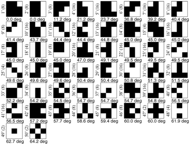
Image 1
CC-BY · From the PDF
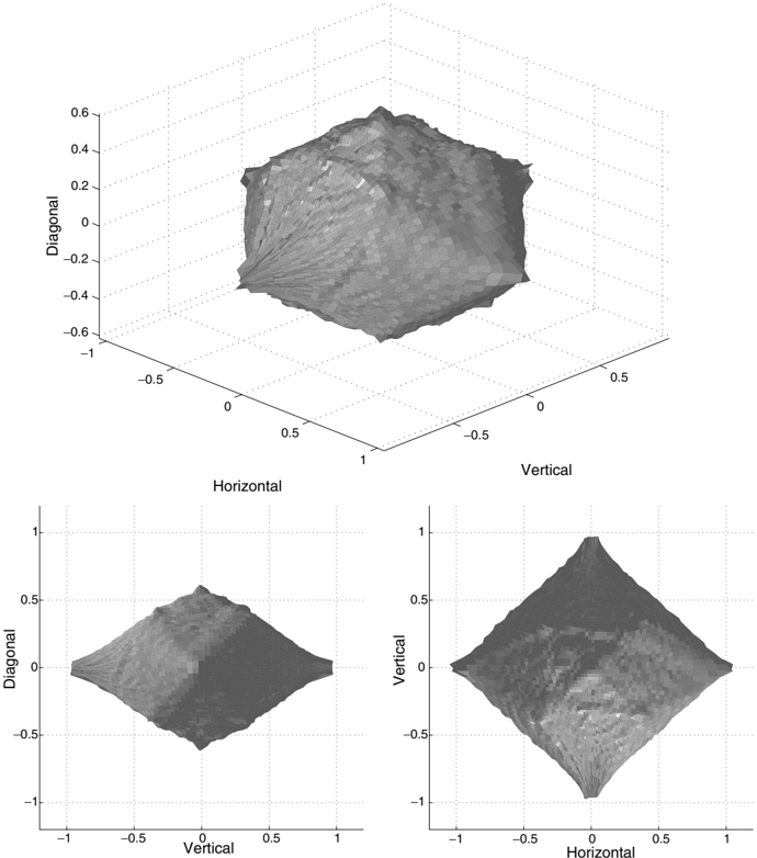
Figure 1 An equi-probable surface of the joint distribution of horizontal, vertical, and diagonal wavelet coefficients in optical images, viewed from three different angles.
Figure 1 An equi-probable surface of the joint distribution of horizontal, vertical, and diagonal wavelet coefficients in optical images, viewed from three different angles.CC-BY · From the PDF
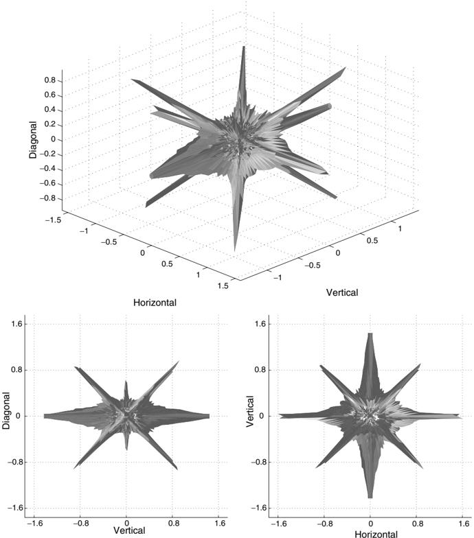
Figure 2 An equi-probable surface of the joint distribution of horizontal, vertical, and diagonal wavelet coefficients in range images, viewed from three different angles.
Figure 2 An equi-probable surface of the joint distribution of horizontal, vertical, and diagonal wavelet coefficients in range images, viewed from three different angles.CC-BY · From the PDF
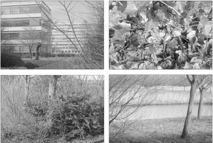
Figure 3 Samples from the van Hateren optical image database. The gray values code for log-intensity values.
Figure 3 Samples from the van Hateren optical image database. The gray values code for log-intensity values.CC-BY · From the PDF
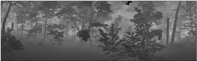
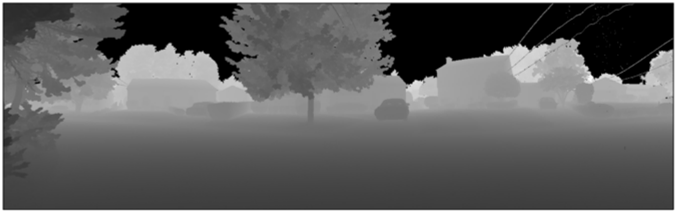
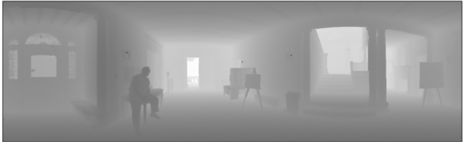
Figure 4 Samples from the Brown range image database by Huang and Lee. The gray values code for log-range values.
Figure 4 Samples from the Brown range image database by Huang and Lee. The gray values code for log-range values.CC-BY · From the PDF
Image 6
CC-BY · From the PDF
Image 7
CC-BY · From the PDF
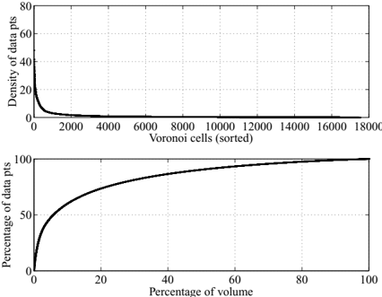
Figure 5 Top: Density ρ ( Omega1 i ) of high-contrast optical patches in Voronoi cells that are sorted according to decreasing density. Bottom: Cumulative percentage of optical patches in the Voronoi cells above versus the cumulative percentage of volume in S 7 that are occupied by these cells.
Figure 5 Top: Density ρ ( Omega1 i ) of high-contrast optical patches in Voronoi cells that are sorted according to decreasing density. Bottom: Cumulative percentage of optical patches in the Voronoi cells above versus the cumulative percentage of volume in S 7 that are occupied by these cells.CC-BY · From the PDF
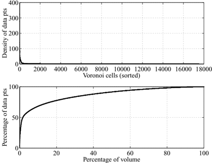
Figure 6 Top: Density ρ ( Omega1 i ) of high-contrast range patches in Voronoi cells that are sorted according to decreasing density. Bottom: Cumulative percentage of range patches in the Voronoi cells above versus the cumulative percentage of volume in S 7 that are occupied by these cells.
Figure 6 Top: Density ρ ( Omega1 i ) of high-contrast range patches in Voronoi cells that are sorted according to decreasing density. Bottom: Cumulative percentage of range patches in the Voronoi cells above versus the cumulative percentage of volume in S 7 that are occupied by these cells.CC-BY · From the PDF
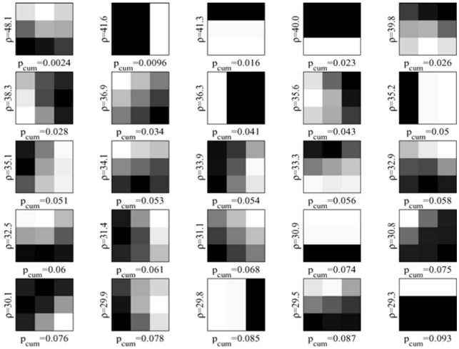
Figure 7 The first 25 Voronoi patches ordered after their densities ρ ( Omega1 i ) in Eq. (12) for optical images. For each Voronoi cell, we display the 3 × 3 patch corresponding to the sample point P i . The cumulative sum of p ( Omega1 i ) (Eq. (13)) over the ordered patches is shown as p cum.
Figure 7 The first 25 Voronoi patches ordered after their densities ρ ( Omega1 i ) in Eq. (12) for optical images. For each Voronoi cell, we display the 3 × 3 patch corresponding to the sample point P i . The cumulative sum of p ( Omega1 i ) (Eq. (13)) over the ordered patches is shown as p cum.CC-BY · From the PDF
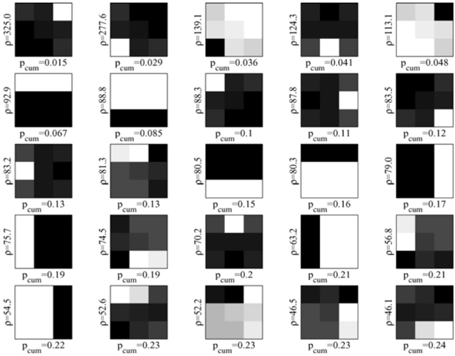
Figure 8 The first 25 Voronoi patches ordered after their densities ρ ( Omega1 i ) in Eq. (12) for range images. For each Voronoi cell, we display the 3 × 3 patch corresponding to the sample point P i . The cumulative sum of p ( Omega1 i ) (Eq. (13)) over the ordered patches is shown as p cum.
Figure 8 The first 25 Voronoi patches ordered after their densities ρ ( Omega1 i ) in Eq. (12) for range images. For each Voronoi cell, we display the 3 × 3 patch corresponding to the sample point P i . The cumulative sum of p ( Omega1 i ) (Eq. (13)) over the ordered patches is shown as p cum.CC-BY · From the PDF
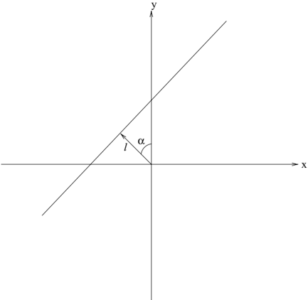
Figure 9 The parameter α ∈ [0 , 2 π ) is the angle that the direction perpendicular to the edge makes with the y-axis, and the parameter l ∈ ( -3 / 2 , 3 / 2) is the displacement of the edge from the origin.
Figure 9 The parameter α ∈ [0 , 2 π ) is the angle that the direction perpendicular to the edge makes with the y-axis, and the parameter l ∈ ( -3 / 2 , 3 / 2) is the displacement of the edge from the origin.CC-BY · From the PDF
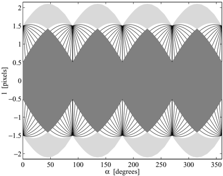
Figure 10 Because of the contrast normalization, some ( α, l )-values are degenerate, i.e. they correspond to the same point v α, l on the 7-dimensional unit sphere S 7 . Each line in the figure is an example of a set of ( α, l )-values that lead to the same contrast-normalized 3 × 3patch. The light shaded region corresponds to degenerate values for corner edges. The dark shaded region in the interior of the graph shows all ( α, l )-values that are well-defined, i.e. non-degenerate.
Figure 10 Because of the contrast normalization, some ( α, l )-values are degenerate, i.e. they correspond to the same point v α, l on the 7-dimensional unit sphere S 7 . Each line in the figure is an example of a set of ( α, l )-values that lead to the same contrast-normalized 3 × 3patch. The light shaded region corresponds to degenerate values for corner edges. The dark shaded region in the interior of the graph shows all ( α, l )-values that are well-defined, i.e. non-degenerate.CC-BY · From the PDF
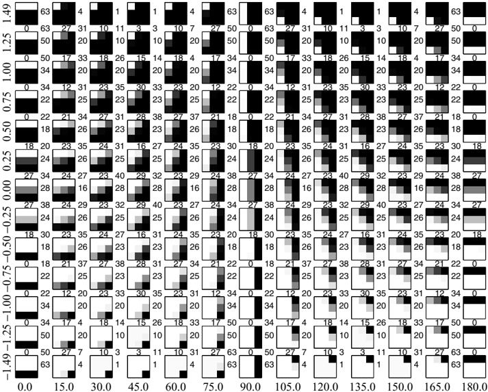
Figure 11 Examples of ideal step edges between 0 ≤ α ≤ 180 degrees (horizontal axis) and 1 . 5 < l < -1 . 5 (vertical axis). The step edges are here chosen on a triangular grid with sides Delta1α = 15 degrees and Delta1 l = 1/4 pixel units. Numbers between patches represent the angular distances in degrees between neighbors in the horizontal, vertical and (lower left-upper right) diagonal directions in the ( α, l )-grid.
Figure 11 Examples of ideal step edges between 0 ≤ α ≤ 180 degrees (horizontal axis) and 1 . 5 < l < -1 . 5 (vertical axis). The step edges are here chosen on a triangular grid with sides Delta1α = 15 degrees and Delta1 l = 1/4 pixel units. Numbers between patches represent the angular distances in degrees between neighbors in the horizontal, vertical and (lower left-upper right) diagonal directions in the ( α, l )-grid.CC-BY · From the PDF
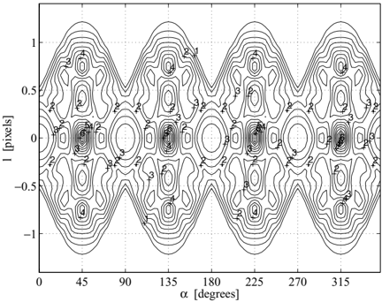
Figure 12 Contour plot of the metric f ( α, l ) = d A d α dl for a surface of ideal step edges. The rectangular bins in the figure have widths Delta1α = π/ 48(3 . 75degrees)and Delta1 l = 1 / 16pixels. For the calculation of the area A of a bin, we add up the areas of 4 or more spherical triangles inside the bin (see text).
Figure 12 Contour plot of the metric f ( α, l ) = d A d α dl for a surface of ideal step edges. The rectangular bins in the figure have widths Delta1α = π/ 48(3 . 75degrees)and Delta1 l = 1 / 16pixels. For the calculation of the area A of a bin, we add up the areas of 4 or more spherical triangles inside the bin (see text).CC-BY · From the PDF
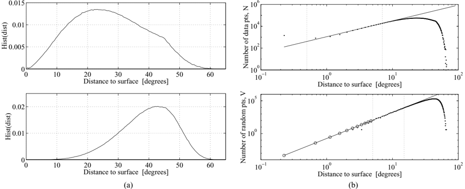
Figure 13 (a) Top : Normalized histogram of the number of optical high-contrast patches, N , versus the distance, θ , to the surface. Bottom : Normalized histogram of the number of random Monte Carlo samples, V , versus θ . (b) Top : Log-log plot of N versus θ . Linear regression in the interval between 0.5 and 7 degrees gives N ∼ θ 1 . 4 (solid line). Bottom : Log-log plot of V versus θ . Linear regression in the interval between 5 and 15 degrees gives V ∼ θ 4 . 0 (solid line). The circles represent extrapolated values of V for θ ≤ 5 degrees. The total number of optical data points is N tot ≈ 4 · 10 6 . The total number of random samples is V tot = 10 7 . The random samples are uniformly distributed on a 7-dimensional unit sphere, and give a Monte Carlo estimate of the volume of the space occupied by the histogram bins.
Figure 13 (a) Top : Normalized histogram of the number of optical high-contrast patches, N , versus the distance, θ , to the surface. Bottom : Normalized histogram of the number of random Monte Carlo samples, V , versus θ . (b) Top : Log-log plot of N versus θ . Linear regression in the interval between 0.5 and 7 degrees gives N ∼ θ 1 . 4 (solid line). Bottom : Log-log plot of V versus θ . Linear regression in the interval between 5 and 15 degrees gives V ∼ θ 4 . 0 (solid line). The circles represent extrapolated values of V for θ ≤ 5 degrees. The total number of optical data points is N tot ≈ 4 · 10 6 . The total number of random samples is V tot = 10 7 . The random samples are uniformly distributed on a 7-dimensional unit sphere, and give a Monte Carlo estimate of the volume of the space occupied by the histogram bins.CC-BY · From the PDF
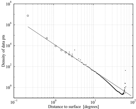
Figure 14 Log-log plot of the average density function p ( θ ) for optical data. For θ < ∼ 10 degrees, p ( θ ) ∼ θ -2 . 5 (solid line). The circles represent the values of the ratio N ( θ ) / N tot V ( θ ) / V tot for extrapolated values of V ( θ ) when θ is small (Fig. 13(b), bottom).
Figure 14 Log-log plot of the average density function p ( θ ) for optical data. For θ < ∼ 10 degrees, p ( θ ) ∼ θ -2 . 5 (solid line). The circles represent the values of the ratio N ( θ ) / N tot V ( θ ) / V tot for extrapolated values of V ( θ ) when θ is small (Fig. 13(b), bottom).CC-BY · From the PDF
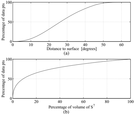
Figure 15 (a) Percentage of optical data points that are within a tubular neighborhood K θ of the surface with width θ ('distance to surface'). (b) Same curve plotted versus the ratio 100 · vol( K θ ) vol(S 7 ) ('percentage of volume of S 7 ').
Figure 15 (a) Percentage of optical data points that are within a tubular neighborhood K θ of the surface with width θ ('distance to surface'). (b) Same curve plotted versus the ratio 100 · vol( K θ ) vol(S 7 ) ('percentage of volume of S 7 ').CC-BY · From the PDF
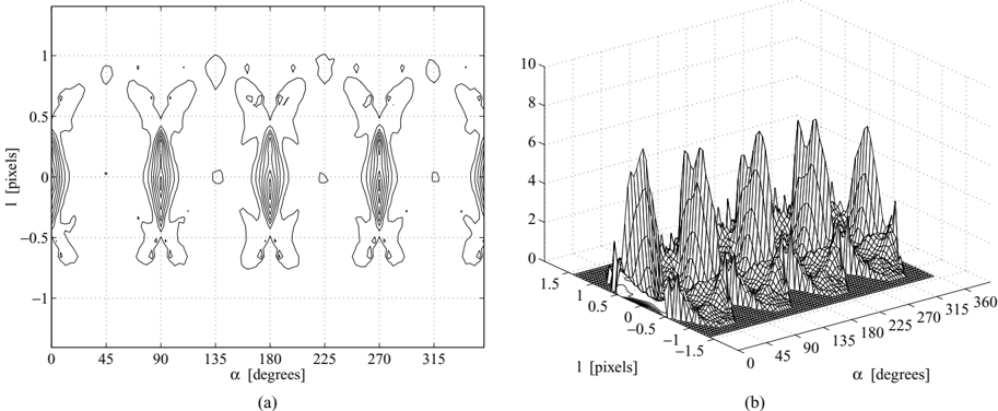
Figure 16 (a) Two-dimensional contour plot and (b) three-dimensional mesh of the density p ( α, l ) of high-contrast optical data along the surface of step edges. In the density calculation, we only include data points that are, at a position ( α, l ) where f ( α, l ) > 0 . 5, and in a tubular neighborhood of the surface with width θ max = 20 degrees. The bin widths Delta1α = π/ 48 (3.75 degrees) and Delta1 l = 1 / 16 pixel units.
Figure 16 (a) Two-dimensional contour plot and (b) three-dimensional mesh of the density p ( α, l ) of high-contrast optical data along the surface of step edges. In the density calculation, we only include data points that are, at a position ( α, l ) where f ( α, l ) > 0 . 5, and in a tubular neighborhood of the surface with width θ max = 20 degrees. The bin widths Delta1α = π/ 48 (3.75 degrees) and Delta1 l = 1 / 16 pixel units.CC-BY · From the PDF
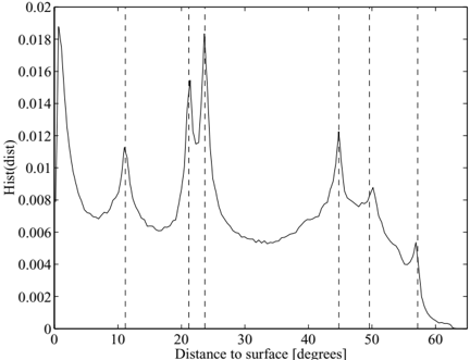
Figure 17 Normalized histogram of N ( θ ) for range patches versus the distance θ to the surface of ideal step edges. Dashed lines corresponds to binary symmetry classes 3 ′ , 4 ′ , 5 ′ , 14 ′ / 18 ′ , 25 ′ , and 42 ′ (see Fig. 18).
Figure 17 Normalized histogram of N ( θ ) for range patches versus the distance θ to the surface of ideal step edges. Dashed lines corresponds to binary symmetry classes 3 ′ , 4 ′ , 5 ′ , 14 ′ / 18 ′ , 25 ′ , and 42 ′ (see Fig. 18).CC-BY · From the PDF
Figure 18 The 50 symmetry classes of binary patches arranged according to increasing θ -values, where θ is the angular distance to the closest point on the surface of ideal step edges. The number below each displayed patch represents this distance. The number in parenthesis left of each patch represents the number of binary patches in each equivalence class.
Figure 18 The 50 symmetry classes of binary patches arranged according to increasing θ -values, where θ is the angular distance to the closest point on the surface of ideal step edges. The number below each displayed patch represents this distance. The number in parenthesis left of each patch represents the number of binary patches in each equivalence class.CC-BY · From the PDF
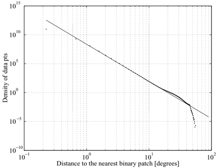
Figure 19 Log-log plot of the density p ( θ ) (Eq. (34)) of highcontrast range patches with respect to θ , the distance to the nearest binary patch. Linear regression in the interval 0 . 6 and 10 degrees gives p ( θ ) ∼ θ -6 . 4 (see solid line).
Figure 19 Log-log plot of the density p ( θ ) (Eq. (34)) of highcontrast range patches with respect to θ , the distance to the nearest binary patch. Linear regression in the interval 0 . 6 and 10 degrees gives p ( θ ) ∼ θ -6 . 4 (see solid line).CC-BY · From the PDF
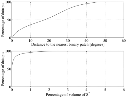
Figure 20 Top: The cumulative percentage P cum( θ ) of the number of patches N ( θ ) with respect to the distance θ to the nearest binary patch. Bottom: The cumulative volume V cum( θ ) versus P cum( θ ).
Figure 20 Top: The cumulative percentage P cum( θ ) of the number of patches N ( θ ) with respect to the distance θ to the nearest binary patch. Bottom: The cumulative volume V cum( θ ) versus P cum( θ ).CC-BY · From the PDF
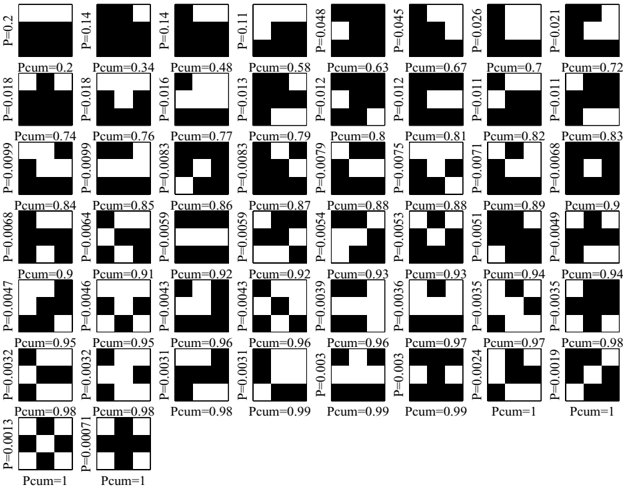
Figure 21 The 50 symmetry classes of binary patches ordered after the percentage Pk ′ of high-contrast range patches closest to one of the binary patches in the equivalence class [ b k ′ ] G . The cumulative percentage Pk ′ , cum is also indicated. For each class, we display the binary patch which is most common among the high-contrast range patches.
Figure 21 The 50 symmetry classes of binary patches ordered after the percentage Pk ′ of high-contrast range patches closest to one of the binary patches in the equivalence class [ b k ′ ] G . The cumulative percentage Pk ′ , cum is also indicated. For each class, we display the binary patch which is most common among the high-contrast range patches.CC-BY · From the PDF
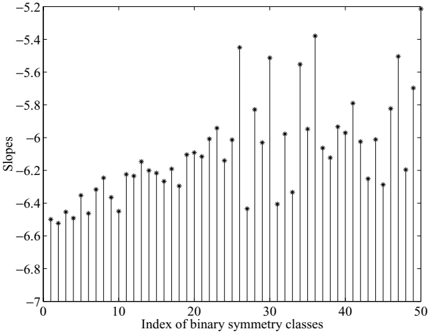
Figure 22 Slopes in a log-log plot of the densities pk ′ ( θ ) for each of the 50 binary symmetry classes [ b k ′ ] G ordered after decreasing cumulative percentage Pk ′ , cum.
Figure 22 Slopes in a log-log plot of the densities pk ′ ( θ ) for each of the 50 binary symmetry classes [ b k ′ ] G ordered after decreasing cumulative percentage Pk ′ , cum.CC-BY · From the PDF

Verification

Claims the paper makes

The claims and statistics of this paper haven’t been checked yet.

Run the check — free, no account needed. It reads the open-access text and checks the sources it cites.

A few free checks a day · papers already verified open instantly · results are public

Claims other papers make about this one

Each is checked against this paper’s own text: does it say what the citing paper says it does?

Self-check

Percentages, sums and reported differences re-computed from the paper’s own numbers.

The self-check needs the paper’s full text.

Citations

Cites

Show all 33 references

Research works printed but not linked: 3

  1. Gemen, D. and Koloydenko, A. 1999. Invariant statistics and coding of natural microimages. In Proc. of the IEEE Workshop on Statistical and Computational Theories of Vission. Published on the Web.
  2. Marr, D. 1982. Vision. New York: W.H. Freeman.
  3. Wegmann, B. and Zetzsche, C. 1990. Statistical dependence between orientation filter outputs used in an human vision based image code. In Proc. SPIE Visual Comm. and Image Processing, vol. 1360. Lausanne, Switzerland, pp. 909-922.

Cited by

Sorted by citations

See all 234

Metadata

Authors
Lee, A. B., Pedersen, K. S., & Mumford, D.
Affiliations
  • Brown University (US)
  • University of Copenhagen (DK)
Venue
International Journal of Computer Vision
Published
2003-08
Volume
54
Issue
1-3
Pages
83-103
ISSN
  • 0920-5691 (ISSN-L)
  • 1573-1405
OpenAlex
W2120023453
Cited by
234
References
33
Citations by year
2026: 1 · 2025: 1 · 2024: 5 · 2023: 4 · 2022: 5 · 2021: 11 · 2020: 12 · 2019: 10 · 2018: 9 · 2017: 12 · 2016: 10 · 2015: 9 · 2014: 12 · 2013: 11 · 2012: 18
FWCI
10.70
Type
journal article
Language
en
Open access
Locations
  • International Journal of Computer Vision (publishedVersion)
  • Digital Access to Scholarship at Harvard (DASH) (Harvard University) (submittedVersion, cc-by)
  • Research at the University of Copenhagen (University of Copenhagen) (submittedVersion)
Funders
Army Research Office
Topics
  • Physical Sciences › Computer Science › Computer Vision and Pattern Recognition › Image Retrieval and Classification Techniques
  • Physical Sciences › Computer Science › Computer Vision and Pattern Recognition › Advanced Vision and Imaging
  • Physical Sciences › Computer Science › Computer Vision and Pattern Recognition › Image and Signal Denoising Methods
Keywords
natural image statistics, density estimation, low-dimensional manifolds, optical imagery, 3D range images, intrinsic dimension

About these checks

Registry, retraction, Cites and statistics results are computed, not judged, with one exception: a printed reference that no index lists is read once by a model before it counts as a citation error. Claims are extracted by a model and kept only when their quote appears verbatim in the text; each cited source is then checked, with a model’s help, for whether it says what the claim relies on. Those verdicts can be wrong — read the claim’s quote and the cited source before relying on one.

Statistics and arithmetic are recomputed, not judged.

Confidence bands are shown only for fields calibrated on our annotated test set. None is calibrated yet, so no band is shown.

What counts as a claim ›How we measure confidence ›How we check this ›

Are you an author, or do you see a problem with this page? Request a review