

The DOI matches its Crossref record; 71 of the 73 references it cites were found in a registry or an index.
Analog forecasting of extreme-causing weather patterns using deep learning
Open accessAbstract
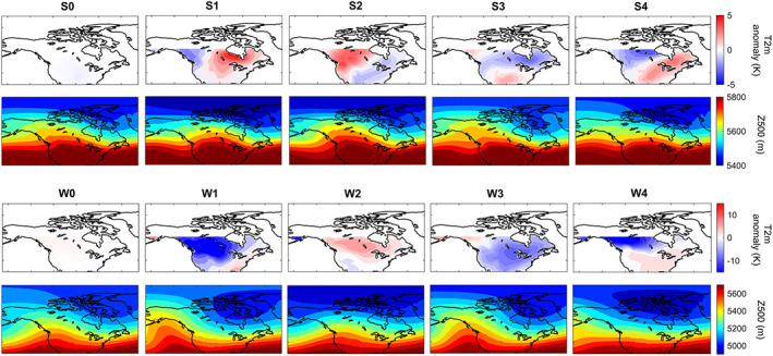
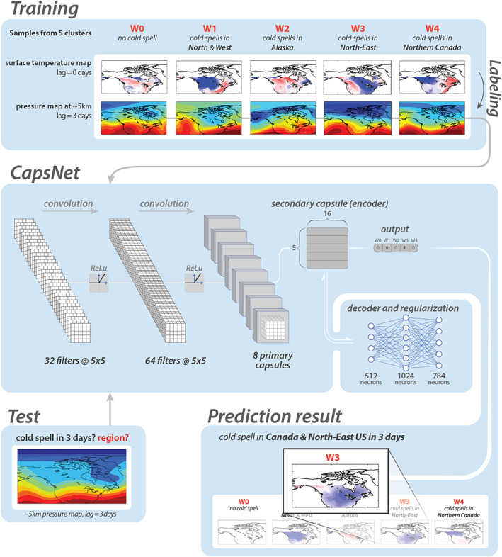
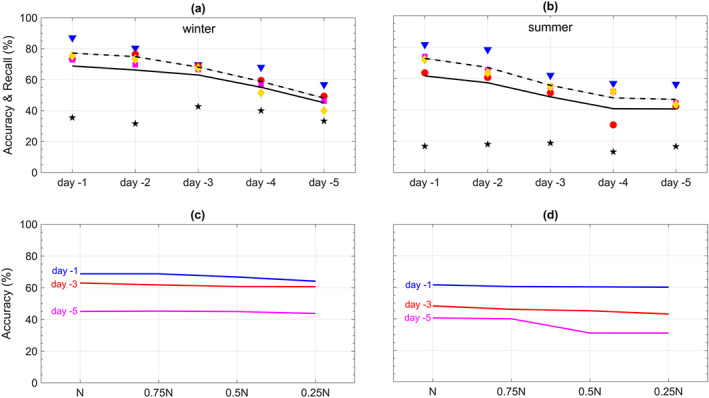
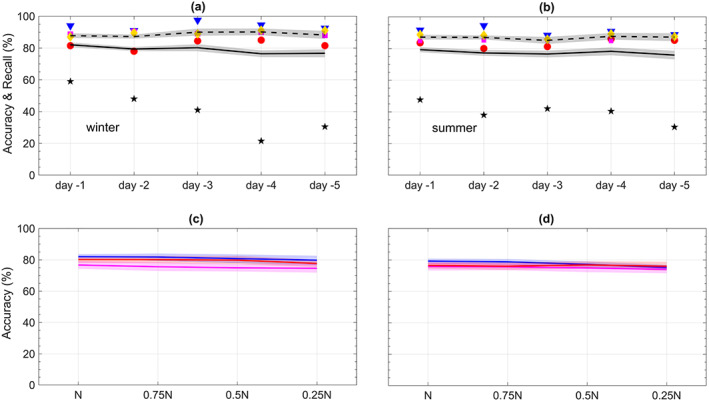
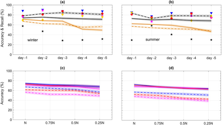
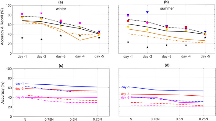
Numerical weather prediction models require ever‐growing computing time and resources but, still, have sometimes difficulties with predicting weather extremes. We introduce a data‐driven framework that is based on analog forecasting (prediction using past similar patterns) and employs a novel deep learning pattern‐recognition technique (capsule neural networks, CapsNets) and an impact‐based autolabeling strategy. Using data from a large‐ensemble fully coupled Earth system model, CapsNets are trained on midtropospheric large‐scale circulation patterns (Z500) labeled 0–4 depending on the existence and geographical region of surface temperature extremes over North America several days ahead. The trained networks predict the occurrence/region of cold or heat waves, only using Z500, with accuracies (recalls) of 69–45% (77–48%) or 62–41% (73–47%) 1–5 days ahead. Using both surface temperature and Z500, accuracies (recalls) with CapsNets increase to 80% (88%). In both cases, CapsNets outperform simpler techniques such as convolutional neural networks and logistic regression, and their accuracy is least affected as the size of the training set is reduced. The results show the promises of multivariate data‐driven frameworks for accurate and fast extreme weather predictions, which can potentially augment numerical weather prediction efforts in providing early warnings.
Overview
The claims and statistics of this paper haven’t been checked yet.
Run the check — free, no account needed. It reads the open-access text and checks the sources it cites.
Integrity signals
Registry
Cites
Statistics
Figures
Verification
Claims the paper makes
The claims and statistics of this paper haven’t been checked yet.
Run the check — free, no account needed. It reads the open-access text and checks the sources it cites.
Claims other papers make about this one
Each is checked against this paper’s own text: does it say what the citing paper says it does?
The source backs part of the claim, not all of it — or backs it for a different population, condition or comparison.
In the citing paper
“While the present is the first to use deep neural network to forecast long-lasting extreme heat waves”
From Deep Learning-Based Extreme Heatwave Forecast (2022) · cites this paper as Chattopadhyay et al., 2020
Experimental — accuracy not yet measured
Self-check
Percentages, sums and reported differences re-computed from the paper’s own numbers.
The self-check needs the paper’s full text.
Citations
Cites
ImageNet classification with deep convolutional neural networks
Krizhevsky, A., Sutskever, I., & Hinton, G. E. (2017) · Communications of the ACM · doi:10.1145/3065386 · Cited by 112,155
Adam: A Method for Stochastic Optimization
Kingma, D. P., & Ba, J. (2014) · arXiv · doi:10.48550/arxiv.1412.6980 · Cited by 98,946
LeCun, Y., Bengio, Y., & Hinton, G. (2015) · Nature · doi:10.1038/nature14539 · Cited by 84,126
An introduction to ROC analysis
Fawcett, T. (2006) · Pattern Recognition Letters · doi:10.1016/j.patrec.2005.10.010 · Cited by 21,879
Visualizing and understanding convolutional networks
Zeiler, M. D., & Fergus, R. (2014) · Lecture Notes in Computer Science · doi:10.1007/978-3-319-10590-1_53 · Cited by 15,839
Least squares quantization in PCM
Lloyd, S. (1982) · IEEE Transactions on Information Theory · doi:10.1109/tit.1982.1056489 · Cited by 15,836
(2016) · Cited by 11,679
Deep learning and process understanding for data-driven Earth system science
Reichstein, M., Camps-Valls, G., Stevens, B., Jung, M., Denzler, J., Carvalhais, N., & Prabhat (2019) · Nature · doi:10.1038/s41586-019-0912-1 · Cited by 5,673
Dynamic Routing Between Capsules
Sabour, S., Frosst, N., & Hinton, G. E. (2017) · arXiv · doi:10.48550/arxiv.1710.09829 · Cited by 4,167
The quiet revolution of numerical weather prediction
Bauer, P., Thorpe, A., & Brunet, G. (2015) · Nature · doi:10.1038/nature14956 · Cited by 2,729
Research works printed but not linked: 1
- 10.1034/j.1600-0870.1994.t01-2-00006.x · DOI
Cited by
Sorted by citations
Physics-informed machine learning: case studies for weather and climate modelling
Kashinath, K., Mustafa, M., Albert, A., Wu, J., Jiang, C.-H., Esmaeilzadeh, S., Azizzadenesheli, K., Wang, R., Chattopadhyay, A., Singh, A., et al. (2021) · Philosophical Transactions of the Royal Society A Mathematical Physical and Engineering Sciences · doi:10.1098/rsta.2020.0093 · Cited by 755
Self-citationPrediction and projection of heatwaves
Domeisen, D. I. V., Eltahir, E. A. B., Fischer, E. M., Knutti, R., Perkins-Kirkpatrick, S. E., Schär, C., Seneviratne, S. I., Weisheimer, A., & Wernli, H. (2022) · Nature Reviews Earth & Environment · doi:10.1038/s43017-022-00371-z · Cited by 504
Heat Waves: Physical Understanding and Scientific Challenges
Barriopedro, D., García‐Herrera, R., Ordóñez, C., Miralles, D. G., & Salcedo‐Sanz, S. (2023) · Reviews of Geophysics · doi:10.1029/2022rg000780 · Cited by 404
Weyn, J. A., Durran, D. R., & Caruana, R. (2020) · Journal of Advances in Modeling Earth Systems · doi:10.1029/2020ms002109 · Cited by 368
Atmospheric blocking and weather extremes over the Euro-Atlantic sector – a review
Kautz, L.-A., Martius, O., Pfahl, S., Pinto, J. G., Ramos, A. M., Sousa, P. M., & Woollings, T. (2022) · Weather and Climate Dynamics · doi:10.5194/wcd-3-305-2022 · Cited by 337
Metadata
- Authors
- Chattopadhyay, A., Nabizadeh, E., & Hassanzadeh, P.
- Affiliations
- Rice University (US)
- Corresponding author
- Hassanzadeh, Pedram
- Venue
- Journal of Advances in Modeling Earth Systems
- Publisher
- American Geophysical Union (AGU)
- Published
- 2020-02
- Volume
- 12
- Issue
- 2
- Pages
- e2019MS001958-e2019MS001958
- ISSN
- 1942-2466 (ISSN-L)
- PMC
- PMC7375135
- OpenAlex
- W2965580012
- Cited by
- 224
- References
- 73
- Citations by year
- 2026: 21 · 2025: 30 · 2024: 42 · 2023: 34 · 2022: 35 · 2021: 46 · 2020: 16
- FWCI
- 10.73
- Type
- journal article
- Language
- en
- Open access
- gold
- doi.org
- Licence
- Locations
- Journal of Advances in Modeling Earth Systems (publishedVersion, cc-by)
- PubMed Central (publishedVersion, cc-by)
- PubMed (publishedVersion)
- EarthArXiv (California Digital Library) (submittedVersion)
- arXiv (Cornell University) (submittedVersion)
- DOAJ (DOAJ: Directory of Open Access Journals) (submittedVersion, cc-by-sa)
- EarthArXiv (OSF Preprints) (submittedVersion)
- Zenodo (CERN European Organization for Nuclear Research) (submittedVersion, cc-by)
- arXiv (Cornell University)
- Funders
- Gulf Research Program
- National Aeronautics and Space Administration (80NSSC17K0266)
- Topics
- Physical Sciences › Earth and Planetary Sciences › Atmospheric Science › Meteorological Phenomena and Simulations
- Physical Sciences › Environmental Science › Global and Planetary Change › Climate variability and models
- Physical Sciences › Environmental Science › Environmental Engineering › Hydrological Forecasting Using AI
- Keywords
- analog forecasting, extreme weather prediction, cold waves, heat waves, capsule networks, Earth system model ensembles, early warning
About these checks
Registry, retraction, Cites and statistics results are computed, not judged, with one exception: a printed reference that no index lists is read once by a model before it counts as a citation error. Claims are extracted by a model and kept only when their quote appears verbatim in the text; each cited source is then checked, with a model’s help, for whether it says what the claim relies on. Those verdicts can be wrong — read the claim’s quote and the cited source before relying on one.
Statistics and arithmetic are recomputed, not judged.
Confidence bands are shown only for fields calibrated on our annotated test set. None is calibrated yet, so no band is shown.
What counts as a claim ›How we measure confidence ›How we check this ›
Are you an author, or do you see a problem with this page? Request a review
