Student or educator? Sign up with your school email and get 6 months of Pro free.
Cited by 211

The DOI matches its Crossref record; 62 of the 62 references it cites were found in a registry or an index.

Late Quaternary dynamics of Arctic biota from ancient environmental genomics

Wang, Yucheng, Pedersen, Mikkel Winther, Alsos, Inger Greve, De Sanctis, Bianca, Racimo, Fernando, Prohaska, Ana, Coissac, Eric, Owens, Hannah Lois, Merkel, Marie Kristine Føreid, Fernandez-Guerra, Antonio, Rouillard, Alexandra, Lammers, Youri, Alberti, Adriana, Denoeud, France, Money, Daniel, Ruter, Anthony H., McColl, Hugh, Larsen, Nicolaj Krog, Cherezova, Anna A., Edwards, Mary E., Fedorov, Grigory B., Haile, James, Orlando, Ludovic, Vinner, Lasse, Korneliussen, Thorfinn Sand, Beilman, David W., Bjørk, Anders A., Cao, Jialu, Dockter, Christoph, Esdale, Julie, Gusarova, Galina, Kjeldsen, Kristian K., Mangerud, Jan, Rasic, Jeffrey T., Skadhauge, Birgitte, Svendsen, John Inge, Tikhonov, Alexei, Wincker, Patrick, Xing, Yingchun, Zhang, Yubin, Froese, Duane G., Rahbek, Carsten, Bravo, David Nogues, Holden, Philip B., Edwards, Neil R., Durbin, Richard, Meltzer, David J., Kjær, Kurt H., Möller, Per, Willerslev, Eske·2021·Nature

Abstract

During the last glacial–interglacial cycle, Arctic biotas experienced substantial climatic changes, yet the nature, extent and rate of their responses are not fully understood 1–8 . Here we report a large-scale environmental DNA metagenomic study of ancient plant and mammal communities, analysing 535 permafrost and lake sediment samples from across the Arctic spanning the past 50,000 years. Furthermore, we present 1,541 contemporary plant genome assemblies that were generated as reference sequences. Our study provides several insights into the long-term dynamics of the Arctic biota at the circumpolar and regional scales. Our key findings include: (1) a relatively homogeneous steppe–tundra flora dominated the Arctic during the Last Glacial Maximum, followed by regional divergence of vegetation during the Holocene epoch; (2) certain grazing animals consistently co-occurred in space and time; (3) humans appear to have been a minor factor in driving animal distributions; (4) higher effective precipitation, as well as an increase in the proportion of wetland plants, show negative effects on animal diversity; (5) the persistence of the steppe–tundra vegetation in northern Siberia enabled the late survival of several now-extinct megafauna species, including the woolly mammoth until 3.9 ± 0.2 thousand years ago (ka) and the woolly rhinoceros until 9.8 ± 0.2 ka; and (6) phylogenetic analysis of mammoth environmental DNA reveals a previously unsampled mitochondrial lineage. Our findings highlight the power of ancient environmental metagenomics analyses to advance understanding of population histories and long-term ecological dynamics.

Overview

The claims and statistics of this paper haven’t been checked yet.

Run the check — free, no account needed. It reads the open-access text and checks the sources it cites.

A few free checks a day · papers already verified open instantly · results are public

Integrity signals

Registry

Crossref · 10.1038/s41586-021-04016-x

Cites

62 of 62 references verified0 citation errors · 0 not checkable

Statistics

Figures

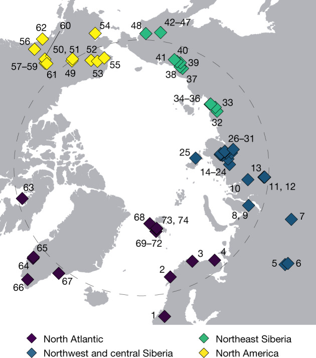
Fig. 1 Site distribution (North Pole-centred view). Samples (n = 535) from a total of 74 circumpolar sites were grouped into four geographical regions (Supplementary Information 2). The grey dashed circle indicates the Arctic Circle (66.5° N). Site IDs are labelled on the map. The corresponding information is provided in Supplementary Data 1.
Fig. 1 Site distribution (North Pole-centred view). Samples (n = 535) from a total of 74 circumpolar sites were grouped into four geographical regions (Supplementary Information 2). The grey dashed circle indicates the Arctic Circle (66.5° N). Site IDs are labelled on the map. The corresponding information is provided in Supplementary Data 1.CC BY · PubMed Central
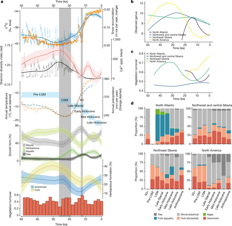
Fig. 2 Climate and vegetation changes over the past 50 kyr. a, Pan-Arctic climate changes and vegetation variations. LGM (26.5−19 ka) and Younger Dryas (YD) (12.9−11.7 ka) are indicated by grey bars. The six time intervals are indicated by light blue bars (Supplementary Information 2). The error bands denote s.e. From top to bottom (see Methods for detailed calculations): the Greenlandic ice-core δ18O ratio and snow accumulation rate; the plant Shannon diversity and the Greenlandic ice-core calcium concentration; the average modelled annual temperature and precipitation for all eDNA sampling sites; the proportion of plant growth forms; the proportion of the herbaceous plant growth forms; and the vegetation turnover rates. b, The number of observed genera in different regions. c, Regional vegetation turnovers. d, Regional vegetation morphological compositions. The sample sizes for each region and time interval are provided in Supplementary Information 2. Calculations are supplied in the Methods.
Fig. 2 Climate and vegetation changes over the past 50 kyr. a, Pan-Arctic climate changes and vegetation variations. LGM (26.5−19 ka) and Younger Dryas (YD) (12.9−11.7 ka) are indicated by grey bars. The six time intervals are indicated by light blue bars (Supplementary Information 2). The error bands denote s.e. From top to bottom (see Methods for detailed calculations): the Greenlandic ice-core δ18O ratio and snow accumulation rate; the plant Shannon diversity and the Greenlandic ice-core calcium concentration; the average modelled annual temperature and precipitation for all eDNA sampling sites; the proportion of plant growth forms; the proportion of the herbaceous plant growth forms; and the vegetation turnover rates. b, The number of observed genera in different regions. c, Regional vegetation turnovers. d, Regional vegetation morphological compositions. The sample sizes for each region and time interval are provided in Supplementary Information 2. Calculations are supplied in the Methods.CC BY · PubMed Central
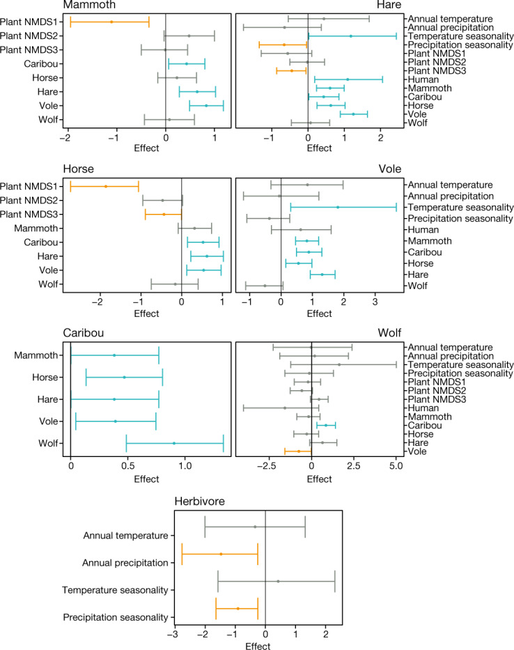
Fig. 3 Spatiotemporal models to retrodict the explanatory factors for animal distribution. The values indicate posterior parameter estimates of covariate effects for the models explaining the presence–absence of each animal’s eDNA. Only covariates included in the model with lowest Watanabe–Aikaike information criterion are shown (Methods). The dots represent the posterior means, and the whiskers represent the posterior 2.5% and 97.5% quantiles. Covariate effects of which the 2.5% and 97.5% quantiles are both negative (red), and effects of which the 2.5% and 97.5% quantiles are both positive (blue) are indicated.
Fig. 3 Spatiotemporal models to retrodict the explanatory factors for animal distribution. The values indicate posterior parameter estimates of covariate effects for the models explaining the presence–absence of each animal’s eDNA. Only covariates included in the model with lowest Watanabe–Aikaike information criterion are shown (Methods). The dots represent the posterior means, and the whiskers represent the posterior 2.5% and 97.5% quantiles. Covariate effects of which the 2.5% and 97.5% quantiles are both negative (red), and effects of which the 2.5% and 97.5% quantiles are both positive (blue) are indicated.CC BY · PubMed Central
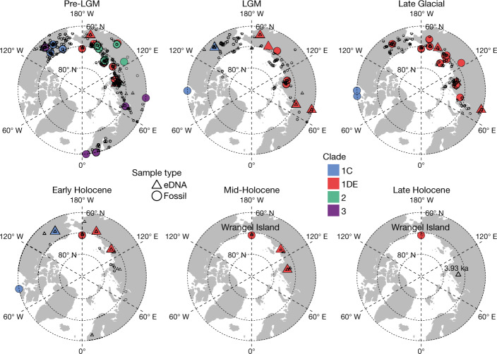
Fig. 4 Mammoth distribution and mitochondrial haplotypes. A total of 78 mammoth mitochondrial genomes and 159 eDNA-identified mammoths (79 among them were assigned to mitochondrial haplotypes) are shown. Records of dated mammoth fossils62 are also plotted. All samples older than 26.5 ka were combined into the pre-LGM interval.
Fig. 4 Mammoth distribution and mitochondrial haplotypes. A total of 78 mammoth mitochondrial genomes and 159 eDNA-identified mammoths (79 among them were assigned to mitochondrial haplotypes) are shown. Records of dated mammoth fossils62 are also plotted. All samples older than 26.5 ka were combined into the pre-LGM interval.CC BY · PubMed Central
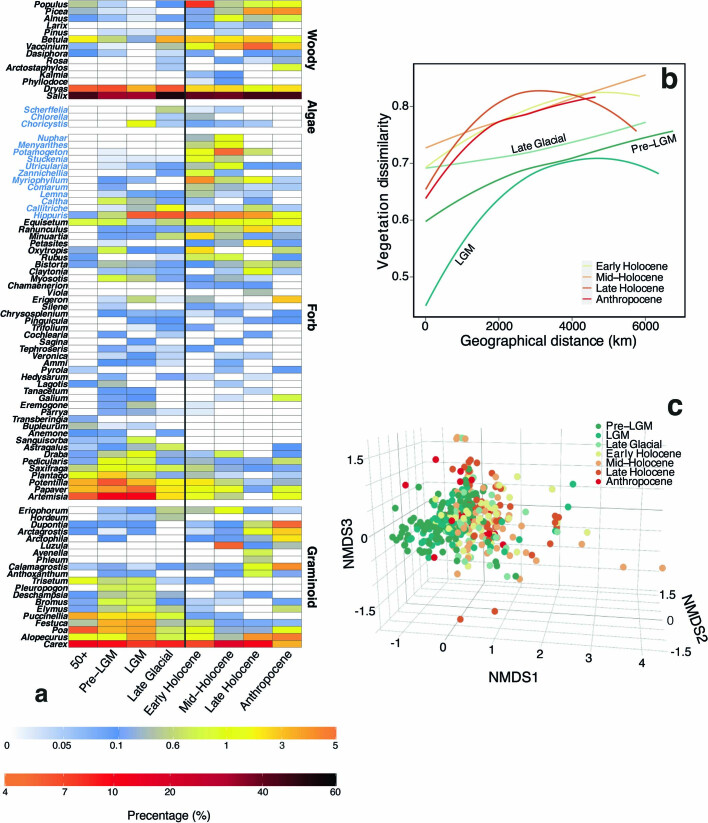
Extended Data Fig. 1 Circum-Arctic plant abundance variations and vegetation similarity clustering. a, Pan-Arctic plant abundance heatmap. b, Spatial vegetation dissimilarities. Pairwise spatial beta-diversities (dissimilarities between every two plant communities) against the geographical distances between the two communities. c, Non-metric Multidimensional Scaling (NMDS, k=3) on vegetation communities.
Extended Data Fig. 1 Circum-Arctic plant abundance variations and vegetation similarity clustering. a, Pan-Arctic plant abundance heatmap. b, Spatial vegetation dissimilarities. Pairwise spatial beta-diversities (dissimilarities between every two plant communities) against the geographical distances between the two communities. c, Non-metric Multidimensional Scaling (NMDS, k=3) on vegetation communities.CC BY · PubMed Central
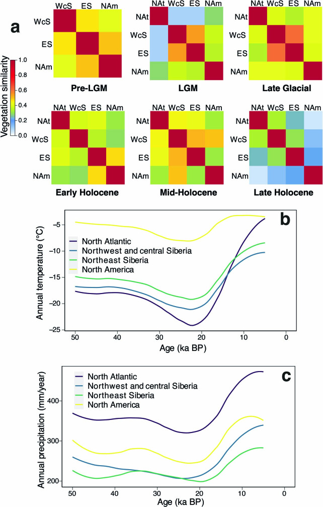
Extended Data Fig. 2 Regional vegetation differences and climate changes. a, Vegetation similarities between each two regions. All identified plant genera across sites in a region during a time interval were merged as a plant assemblage. Spatial beta-diversity between every two assemblages were calculated and illustrated. NAt, North Atlantic; WcS, Northwest and central Siberia; ES, Northeast Siberia; Nam, North America. b and c, Modelled annual temperature and precipitation in different regions. Means of the modelled annual temperature and precipitation values (Methods) at all eDNA sampling sites within a region at each 1,000-year time step were calculated. The changing trends are illustrated.
Extended Data Fig. 2 Regional vegetation differences and climate changes. a, Vegetation similarities between each two regions. All identified plant genera across sites in a region during a time interval were merged as a plant assemblage. Spatial beta-diversity between every two assemblages were calculated and illustrated. NAt, North Atlantic; WcS, Northwest and central Siberia; ES, Northeast Siberia; Nam, North America. b and c, Modelled annual temperature and precipitation in different regions. Means of the modelled annual temperature and precipitation values (Methods) at all eDNA sampling sites within a region at each 1,000-year time step were calculated. The changing trends are illustrated.CC BY · PubMed Central
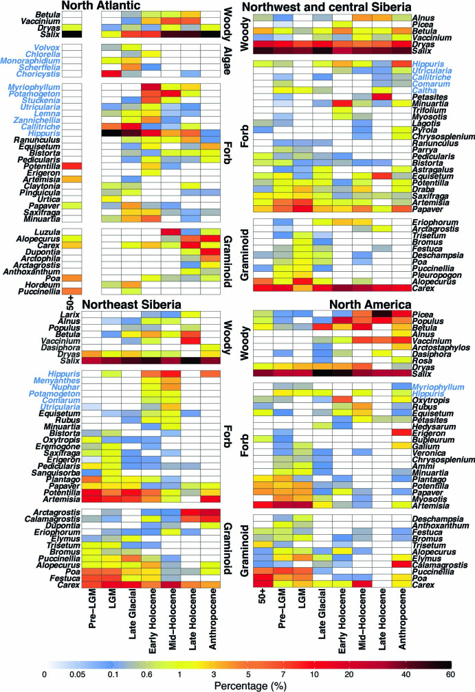
Extended Data Fig. 3 Regional plant abundance heatmaps. Heatmaps show the relative abundances of the 40 abundant plant genera in each region.
Extended Data Fig. 3 Regional plant abundance heatmaps. Heatmaps show the relative abundances of the 40 abundant plant genera in each region.CC BY · PubMed Central
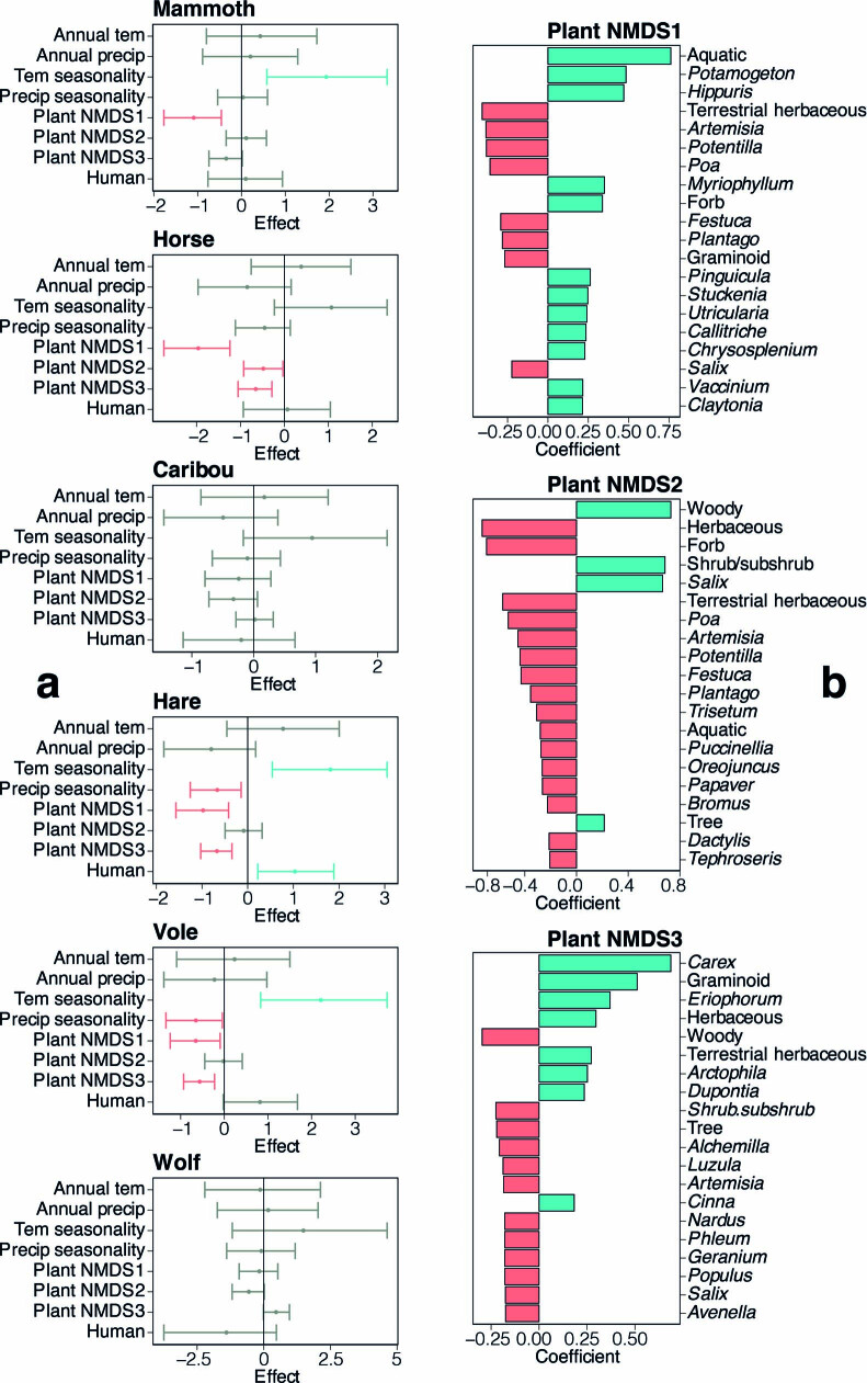
Extended Data Fig. 4 Environmental explanatory factors for animal distribution, and plant NMDS components. a, Posterior parameter estimates of covariate effects for the models explaining the presence/absence of each animal’s eDNA using climate, human presence and plant NMDS as explanatory variables. The dots represent the posterior means, and the whiskers represent the posterior 2.5% and 97.5% quantiles. The colour red denotes covariate effects whose 2.5% and 97.5% quantiles are both negative, while the colour blue denotes covariate effects 2.5% and 97.5% quantiles are both positive. b, The plant genera and morphological forms correlated to the 3 components of plant NMDS. Plant genera (morphological forms) are ranked by the p-value of t-test, and only the top 20 Pearson correlations are shown. The colour red denotes negative correlations while the colour blue denotes positive correlations.
Extended Data Fig. 4 Environmental explanatory factors for animal distribution, and plant NMDS components. a, Posterior parameter estimates of covariate effects for the models explaining the presence/absence of each animal’s eDNA using climate, human presence and plant NMDS as explanatory variables. The dots represent the posterior means, and the whiskers represent the posterior 2.5% and 97.5% quantiles. The colour red denotes covariate effects whose 2.5% and 97.5% quantiles are both negative, while the colour blue denotes covariate effects 2.5% and 97.5% quantiles are both positive. b, The plant genera and morphological forms correlated to the 3 components of plant NMDS. Plant genera (morphological forms) are ranked by the p-value of t-test, and only the top 20 Pearson correlations are shown. The colour red denotes negative correlations while the colour blue denotes positive correlations.CC BY · PubMed Central
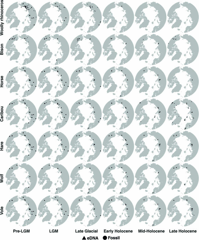
Extended Data Fig. 5 Distribution chronologies for woolly rhinoceros, bison, horse, caribou, hare, wolf, and vole. We combined our DNA results and the fossil records62 (available for woolly rhinoceros, bison, and caribou). Samples older than 26.5 ka were combined into Pre-LGM; samples younger than 4.2 ka were combined into the Late Holocene.
Extended Data Fig. 5 Distribution chronologies for woolly rhinoceros, bison, horse, caribou, hare, wolf, and vole. We combined our DNA results and the fossil records62 (available for woolly rhinoceros, bison, and caribou). Samples older than 26.5 ka were combined into Pre-LGM; samples younger than 4.2 ka were combined into the Late Holocene.CC BY · PubMed Central
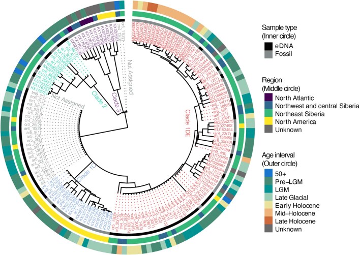
Extended Data Fig. 6 Mammoth mitochondrial phylogenetic tree. For placed eDNA samples the number of supporting single-nucleotide polymorphisms is given in braces (Methods). IDs for the Wrangel Island population are underlined.
Extended Data Fig. 6 Mammoth mitochondrial phylogenetic tree. For placed eDNA samples the number of supporting single-nucleotide polymorphisms is given in braces (Methods). IDs for the Wrangel Island population are underlined.CC BY · PubMed Central

Verification

Claims the paper makes

The claims and statistics of this paper haven’t been checked yet.

Run the check — free, no account needed. It reads the open-access text and checks the sources it cites.

A few free checks a day · papers already verified open instantly · results are public

Claims other papers make about this one

Each is checked against this paper’s own text: does it say what the citing paper says it does?

Self-check

Percentages, sums and reported differences re-computed from the paper’s own numbers.

The self-check needs the paper’s full text.

Citations

Cites

Show all 62 references

Cited by

Metadata

Authors
Wang, Y., Pedersen, M. W., Alsos, I. G., De Sanctis, B., Racimo, F., Prohaska, A., Coissac, E., Owens, H. L., Merkel, M. K. F., Fernandez-Guerra, A., Rouillard, A., Lammers, Y., Alberti, A., Denoeud, F., Money, D., Ruter, A. H., McColl, H., Larsen, N. K., Cherezova, A. A., Edwards, M. E., Fedorov, G. B., Haile, J., Orlando, L., Vinner, L., Korneliussen, T. S., Beilman, D. W., Bjørk, A. A., Cao, J., Dockter, C., Esdale, J., Gusarova, G., Kjeldsen, K. K., Mangerud, J., Rasic, J. T., Skadhauge, B., Svendsen, J. I., Tikhonov, A., Wincker, P., Xing, Y., Zhang, Y., Froese, D. G., Rahbek, C., Bravo, D. N., Holden, P. B., Edwards, N. R., Durbin, R., Meltzer, D. J., Kjær, K. H., Möller, P., & Willerslev, E.
Venue
Nature
Published
2021-10-20
Volume
600
Issue
7887
Pages
86-92
ISSN
  • 0028-0836
  • 1476-4687
Cited by
211
References
62
Language
en

About these checks

Registry, retraction, Cites and statistics results are computed, not judged, with one exception: a printed reference that no index lists is read once by a model before it counts as a citation error. Claims are extracted by a model and kept only when their quote appears verbatim in the text; each cited source is then checked, with a model’s help, for whether it says what the claim relies on. Those verdicts can be wrong — read the claim’s quote and the cited source before relying on one.

Statistics and arithmetic are recomputed, not judged.

Confidence bands are shown only for fields calibrated on our annotated test set. None is calibrated yet, so no band is shown.

What counts as a claim ›How we measure confidence ›How we check this ›

Are you an author, or do you see a problem with this page? Request a review

Data sources

Bibliographic data: Semantic Scholar, OpenAlex, Crossref.

Contains information from the Semantic Scholar Academic Graph Datasets, made available under the ODC Attribution License (ODC-BY 1.0).

Semantic Scholar’s data is described in: Kinney, R., et al. (2023). The Semantic Scholar Open Data Platform. arXiv:2301.10140.