

The DOI matches its Crossref record; 5 of the 5 references it cites were found in a registry or an index.
The quantum transition of the two-dimensional Ising spin glass
Open accessAbstract
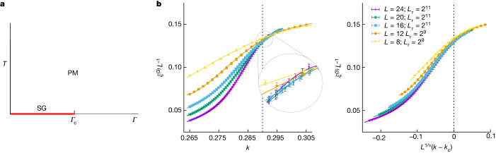
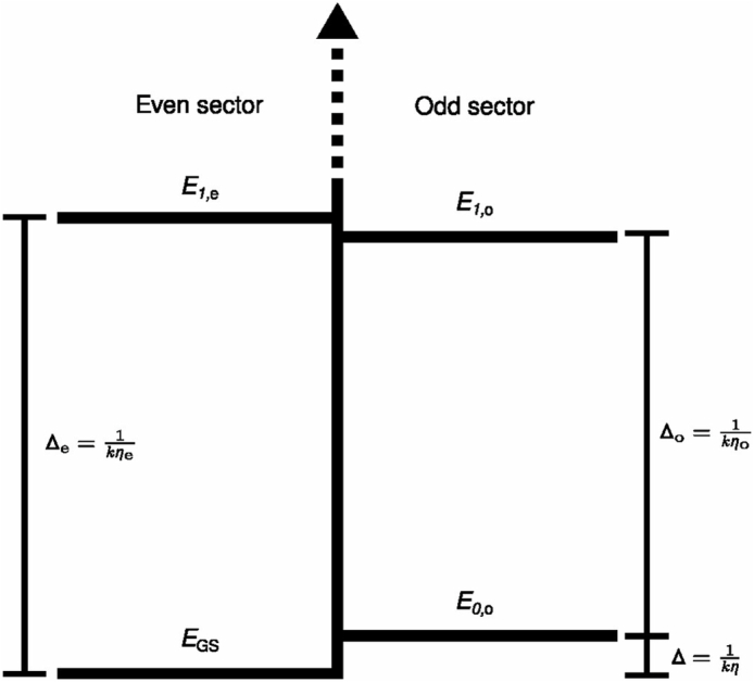
Quantum annealers are commercial devices that aim to solve very hard computational problems 1, typically those involving spin glasses 2,3. Just as in metallurgic annealing, in which a ferrous metal is slowly cooled 4, quantum annealers seek good solutions by slowly removing the transverse magnetic field at the lowest possible temperature. Removing the field diminishes the quantum fluctuations but forces the system to traverse the critical point that separates the disordered phase (at large fields) from the spin-glass phase (at small fields). A full understanding of this phase transition is still missing. A debated, crucial question regards the closing of the energy gap separating the ground state from the first excited state. All hopes of achieving an exponential speed-up, compared to classical computers, rest on the assumption that the gap will close algebraically with the number of spins 5–9. However, renormalization group calculations predict instead that there is an infinite-randomness fixed point 10. Here we solve this debate through extreme-scale numerical simulations, finding that both parties have grasped parts of the truth. Although the closing of the gap at the critical point is indeed super-algebraic, it remains algebraic if one restricts the symmetry of possible excitations. As this symmetry restriction is experimentally achievable (at least nominally), there is still hope for the quantum annealing paradigm 11–13.
Overview
The claims and statistics of this paper haven’t been checked yet.
Run the check — free, no account needed. It reads the open-access text and checks the sources it cites.
Integrity signals
Registry
Cites
Statistics
Figures
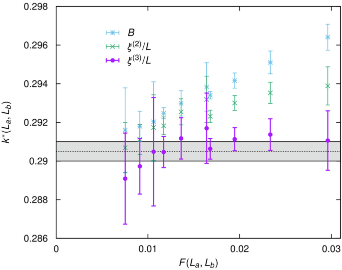
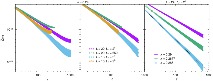
Verification
Claims the paper makes
The claims and statistics of this paper haven’t been checked yet.
Run the check — free, no account needed. It reads the open-access text and checks the sources it cites.
Claims other papers make about this one
Each is checked against this paper’s own text: does it say what the citing paper says it does?
The source backs part of the claim, not all of it — or backs it for a different population, condition or comparison.
In the citing paper
“The authors extracted distinct estimates for the finite-size measurement (fixing their fitting parameter η 0 e = 0) and the large-system limit of, respectively, µ = z + 1/ν = 1.7(2) + 0.9(1) = 2.6(3) (S12) and µ = z + 1/ν = 2.46(17) + 0.71(24) = 3.27( 41),”
From Beyond-classical computation in quantum simulation (2025) · cites this paper as [37]
Experimental — accuracy not yet measuredThe cited source says what the claim attributes to it.
In the citing paper
“For 2D, this was settled very recently 37 through the consideration of distinct parity sectors in the state space, using MC simulations of lowprecision L×L square lattices (with fully periodic boundaries) with L ranging from 8 to 24.”
From Beyond-classical computation in quantum simulation (2025) · cites this paper as [37]
Self-check
Percentages, sums and reported differences re-computed from the paper’s own numbers.
The self-check needs the paper’s full text.
Citations
Cites
Spin Glass Theory and Beyond: An Introduction to the Replica Method and Its Applications
Mezard, M., Parisi, G., & Virasoro, M. (1986) · World Scientific Lecture Notes in Physics · doi:10.1142/0271 · Cited by 3,653
Quantum annealing in the transverse Ising model
Kadowaki, T., & Nishimori, H. (1998) · Physical Review E · doi:10.1103/physreve.58.5355 · Cited by 2,339
On the product of semi-groups of operators
Trotter, H. F. (1959) · Proceedings of the American Mathematical Society · doi:10.1090/s0002-9939-1959-0108732-6 · Cited by 2,282
An introduction to lattice gauge theory and spin systems
Kogut, J. B. (1979) · Reviews of Modern Physics · doi:10.1103/revmodphys.51.659 · Cited by 2,029
Quantum annealing with manufactured spins
Johnson, M. W., Amin, M. H. S., Gildert, S., Lanting, T., Hamze, F., Dickson, N., Harris, R., Berkley, A. J., Johansson, J., Bunyk, P., et al. (2011) · Nature · doi:10.1038/nature10012 · Cited by 1,891
Research works printed but not linked: 72
- Charbonneau, P. et al. (eds) Spin Glass Theory and Far Beyond (World Scientific, 2023). · DOI
- Binder, K. & Young, A. P. Spin glasses: experimental facts, theoretical concepts, and open questions. Rev. Mod. Phys. 58, 801–976 (1986). · DOI
- Kirkpatrick, S., Gelatt, C. D. & Vecchi, M. P. Optimization by simulated annealing. Science 220, 671–680 (1983). · DOI · Paper page
- Rieger, H. & Young, A. P. Zero-temperature quantum phase transition of a two-dimensional Ising spin glass. Phys. Rev. Lett. 72, 4141–4144 (1994). · DOI · Paper page
- Guo, M., Bhatt, R. N. & Huse, D. A. Quantum critical behavior of a three-dimensional Ising spin glass in a transverse magnetic field. Phys. Rev. Lett. 72, 4137–4140 (1994). · DOI · Paper page
- Guo, M., Bhatt, R. N. & Huse, D. A. Quantum Griffiths singularities in the transverse-field Ising spin glass. Phys. Rev. B 54, 3336–3342 (1996). · DOI
- Rieger, H. & Young, A. P. Griffiths singularities in the disordered phase of a quantum Ising spin glass. Phys. Rev. B 54, 3328–3335 (1996). · DOI
- Singh, R. R. P. & Young, A. P. Critical and Griffiths–McCoy singularities in quantum Ising spin glasses on d-dimensional hypercubic lattices: a series expansion study. Phys. Rev. E 96, 022139 (2017). · DOI
- Miyazaki, R. & Nishimori, H. Real-space renormalization-group approach to the random transverse-field Ising model in finite dimensions. Phys. Rev. E 87, 032154 (2013). · DOI
- Brooke, J., Bitko, D., Rosenbaum, & Aeppli, G. Quantum annealing of a disordered magnet. Science 284, 779–781 (1999). · DOI · Paper page
- Farhi, E. et al. A quantum adiabatic evolution algorithm applied to random instances of an NP-complete problem. Science 292, 472–475 (2001). · DOI · Paper page
- Papadimitriou, C. Computational Complexity (Addison-Wesley, 1994).
- Barahona, F. On the computational complexity of Ising spin glass models. J. Phys. A: Math. Gen. 15, 3241 (1982). · DOI
- Istrail, S. Statistical mechanics, three-dimensionality and NP-completeness. I. Universality of intracatability for the partition function of the Ising model across non-planar surfaces (extended abstract). In Proc. 32nd Annual ACM Symposium on Theory of Computing (eds Yao, F. & Luks, E.) 87–96 (ACM, 2000). · DOI
- Goto, H., Tatsumura, K. & Dixon, A. R. Combinatorial optimization by simulating adiabatic bifurcations in nonlinear Hamiltonian systems. Sci. Adv. 5, eaav2372 (2019). · DOI
- Matsubara, S. et al. Digital annealer for high-speed solving of combinatorial optimization problems and its applications. In Proc. 2020 25th Asia and South Pacific Design Automation Conference (ASP-DAC) (eds Cheng, K.-T. T. & Yang, H.) 667–672 (IEEE, 2020). · DOI
- Takemoto, T., Hayashi, M., Yoshimura, C. & Yamaoka, M. A 2 × 30k-spin multi-chip scalable CMOS annealing processor based on a processing-in-memory approach for solving large-scale combinatorial optimization problems. IEEE J. Solid-State Circuits 55, 145–156 (2020). · DOI
- McMahon, P. L. et al. A fully programmable 100-spin coherent Ising machine with all-to-all connections. Science 354, 614–617 (2016). · DOI
- Baity-Jesi, M. et al. Janus II: a new generation application-driven computer for spin-system simulations. Comput. Phys. Commun. 185, 550–559 (2014). · DOI
- King, A. D. et al. Quantum critical dynamics in a 5,000-qubit programmable spin glass. Nature 617, 61–66 (2023). · DOI · Paper page
- Parisi, G. Field Theory, Disorder and Simulations (World Scientific, 1994).
- Grinstein, G. & Luther, A. Application of the renormalization group to phase transitions in disordered systems. Phys. Rev. B 13, 1329–1343 (1976). · DOI
- Parisi, G. Infinite number of order parameters for spin-glasses. Phys. Rev. Lett. 43, 1754–1756 (1979). · DOI · Paper page
- Parisi, G. & Sourlas, N. Random magnetic fields, supersymmetry, and negative dimensions. Phys. Rev. Lett. 43, 744–745 (1979). · DOI
- Cardy, J. Scaling and Renormalization in Statistical Field Theory, Vol. 5 of Lecture Notes in Physics (eds Goddard, P. & Yeomans, J.) (Cambridge Univ. Press, 1996).
- Ballesteros, H. G. et al. Critical exponents of the three-dimensional diluted Ising model. Phys. Rev. B 58, 2740–2747 (1998). · DOI
- Hasenbusch, M., Pelissetto, A. & Vicari, E. Critical behavior of three-dimensional Ising spin glass models. Phys. Rev. B 78, 214205 (2008). · DOI
- Fytas, N. G. & Martín-Mayor, V. Universality in the three-dimensional random-field Ising model. Phys. Rev. Lett. 110, 227201 (2013). · DOI
- Fytas, N. G., Martín-Mayor, V., Picco, M. & Sourlas, N. Phase transitions in disordered systems: the example of the random-field Ising model in four dimensions. Phys. Rev. Lett. 116, 227201 (2016). · DOI
- Fytas, N. G., Martín-Mayor, V., Parisi, G., Picco, M. & Sourlas, N. Evidence for supersymmetry in the random-field Ising model at d = 5. Phys. Rev. Lett. 122, 240603 (2019). · DOI
- Fernandez, L. A., Marinari, E., Martin-Mayor, V., Parisi, G. & Ruiz-Lorenzo, J. J. Universal critical behavior of the two-dimensional Ising spin glass. Phys. Rev. B 94, 024402 (2016). · DOI
- McCoy, B. M. & Wu, T. Theory of a two-dimensional Ising model with random impurities. I. Thermodynamics. Phys. Rev. 176, 631–643 (1968). · DOI
- McCoy, B. M. & Wu, T. Theory of a two-dimensional Ising model with random impurities. II. Spin correlation functions. Phys. Rev. 188, 982–1013 (1969). · DOI
- McCoy, B. M. Theory of a two-dimensional Ising model with random impurities. III. Boundary effects. Phys. Rev. 188, 1014–1031 (1969). · DOI
- Fisher, D. S. Random transverse field Ising spin chains. Phys. Rev. Lett. 69, 534–537 (1992). · DOI
- Albash, T. & Lidar, D. A. Adiabatic quantum computation. Rev. Mod. Phys. 90, 015002 (2018). · DOI · Paper page
- Thill, M. J. & Huse, D. A. Equilibrium behaviour of quantum Ising spin glass. Phys. A: Stat. Mech. Appl. 214, 321–355 (1995). · DOI
- Matoz-Fernandez, D. A. & Romá, F. Unconventional critical activated scaling of two-dimensional quantum spin glasses. Phys. Rev. B 94, 024201 (2016). · DOI
- Griffiths, R. B. Nonanalytic behavior above the critical point in a random Ising ferromagnet. Phys. Rev. Lett. 23, 17–19 (1969). · DOI
- Farhi, E. et al. Performance of the quantum adiabatic algorithm on random instances of two optimization problems on regular hypergraphs. Phys. Rev. A 86, 052334 (2012). · DOI
- Yang, C. N. Concept of off-diagonal long-range order and the quantum phases of liquid He and of superconductors. Rev. Mod. Phys. 34, 694–704 (1962). · DOI
- Sinova, J., Canright, G. & MacDonald, A. H. Nature of ergodicity breaking in Ising spin glasses as revealed by correlation function spectral properties. Phys. Rev. Lett. 85, 2609–2612 (2000). · DOI
- Correale, L., Marinari, E. & Martín-Mayor, V. Eigenvalue analysis of the density matrix of four-dimensional spin glasses supports replica symmetry breaking. Phys. Rev. B 66, 174406 (2002). · DOI
- Amit, D. J. & Martín-Mayor, V. Field Theory, the Renormalization Group and Critical Phenomena 3rd edn (World Scientific, 2005). · DOI
- Chayes, J. T., Chayes, L., Fisher, D. S. & Spencer, T. Finite-size scaling and correlation lengths for disordered systems. Phys. Rev. Lett. 57, 2999–3002 (1986). · DOI
- King, A. D. et al. Computational supremacy in quantum simulation. Preprint at https://arxiv.org/abs/2403.00910 (2024). · arXiv
- Hen, I. & Young, A. P. Exponential complexity of the quantum adiabatic algorithm for certain satisfiability problems. Phys. Rev. E 84, 061152 (2011). · DOI
- Knysh, S. Zero-temperature quantum annealing bottlenecks in the spin-glass phase. Nat. Commun. 7, 12370 (2016). · DOI
- Khoshbakht, H. & Weigel, M. Domain-wall excitations in the two-dimensional Ising spin glass. Phys. Rev. B 97, 064410 (2018). · DOI
- Fernandez, L. A., Martín-Mayor, V., Parisi, G. & Seoane, B. Temperature chaos in 3D Ising spin glasses is driven by rare events. Europhys. Lett. 103, 67003 (2013). · DOI
- Marshall, J., Martin-Mayor, V. & Hen, I. Practical engineering of hard spin-glass instances. Phys. Rev. A 94, 012320 (2016). · DOI
- Billoire, A. et al. Dynamic variational study of chaos: spin glasses in three dimensions. J. Stat. Mech.: Theory Exp. 2018, 033302 (2018). · DOI
- Martín-Mayor, V. & Hen, I. Unraveling quantum annealers using classical hardness. Sci. Rep. 5, 15324 (2015). · DOI
- Albash, T., Martin-Mayor, V. & Hen, I. Temperature scaling law for quantum annealing optimizers. Phys. Rev. Lett. 119, 110502 (2017). · DOI
- Albash, T., Martin-Mayor, V. & Hen, I. Analog errors in Ising machines. Quantum Sci. Technol. 4, 02LT03 (2019). · DOI
- Nightingale, M. P. Scaling theory and finite systems. Phys. A: Stat. Mech. Appl. 83, 561–572 (1976). · DOI · Paper page
- Toulouse, G. Theory of the frustration effect in spin glasses. Commun. Phys. 2, 115–119 (1977).
- Suzuki, M. Relationship between d-dimensional quantal spin systems and (d + 1)-dimensional Ising systems: equivalence, critical exponents and systematic approximants of the partition function and spin correlations. Prog. Theor. Phys. 56, 1454–1469 (1976). · DOI
- Parisi, G. Statistical Field Theory (Addison-Wesley, 1988). · DOI
- Palassini, M. & Caracciolo, S. Universal finite-size scaling functions in the 3D Ising spin glass. Phys. Rev. Lett. 82, 5128–5131 (1999). · DOI
- Ballesteros, H. G. et al. Critical behavior of the three-dimensional Ising spin glass. Phys. Rev. B 62, 14237–14245 (2000). · DOI
- Bernaschi, M., Pemartín, I. G.-A., Martín-Mayor, V. & Parisi, G. The QISG suite: high-performance codes for studying quantum Ising spin glasses. Comput. Phys. Commun. 298, 109101 (2024). · DOI
- Hukushima, K. & Nemoto, K. Exchange Monte Carlo method and application to spin glass simulations. J. Phys. Soc. Jpn 65, 1604 (1996). · DOI
- Efron, B. & Tibshirani, R. J. An Introduction to Bootstrap (Chapman & Hall/CRC, 1994). · DOI · Paper page
- Fisher, M. E. & Ferdinand, A. E. Interfacial, boundary, and size effects at critical points. Phys. Rev. Lett. 19, 169–172 (1967). · DOI
- Fisher, M. E. & Barber, M. N. Scaling theory for finite-size effects in the critical region. Phys. Rev. Lett. 28, 1516–1519 (1972). · DOI
- Barber, M. N. Finite-size Scaling, Vol. 8 of Phase Transitions and Critical Phenomena (Academic Press, 1983).
- Cardy, J. Finite-size Scaling (Elsevier, 2012).
- Ballesteros, H. G., Fernandez, L. A., Martín-Mayor, V. & Muñoz Sudupe, A. New universality class in three dimensions?: The antiferromagnetic RP2 model. Phys. Lett. B 378, 207 (1996). · DOI
- Yllanes, D. Rugged Free-Energy Landscapes in Disordered Spin Systems. PhD thesis, Complutense Univ. of Madrid (2011).
- Binder, K. Finite size scaling analysis of Ising model block distribution functions. Z. Phys. B: Condens. Matter 43, 119–140 (1981). · DOI
- Belletti, F. et al. Nonequilibrium spin-glass dynamics from picoseconds to one tenth of a second. Phys. Rev. Lett. 101, 157201 (2008). · DOI
Cited by
Sorted by citations
Beyond-classical computation in quantum simulation
King, A. D., Nocera, A., Rams, M. M., Dziarmaga, J., Wiersema, R., Bernoudy, W., Raymond, J., Kaushal, N., Heinsdorf, N., Harris, R., et al. (2025) · Science · doi:10.1126/science.ado6285 · Cited by 138
Metadata
- Authors
- Bernaschi, M., González-Adalid Pemartín, I., Martín-Mayor, V., & Parisi, G.
- Affiliations
- Istituto per le Applicazioni del Calcolo Mauro Picone (IT)
- Universidad Complutense de Madrid (ES)
- Venue
- Nature
- Published
- 2024-07-10
- Volume
- 631
- Issue
- 8022
- Pages
- 749-754
- ISSN
- 0028-0836 (ISSN-L)
- 1476-4687
- PMC
- PMC11269196
- OpenAlex
- W4400491633
- Cited by
- 35
- References
- 5
- Citations by year
- 2026: 14 · 2025: 19 · 2024: 2
- FWCI
- 5.05
- Type
- journal article
- Language
- en
- Open access
- hybrid
- doi.org
- Locations
- Nature (publishedVersion, cc-by)
- PubMed Central (publishedVersion, cc-by)
- PubMed (publishedVersion)
- arXiv (Cornell University) (submittedVersion)
- RePEc: Research Papers in Economics (submittedVersion)
- arXiv (Cornell University)
- Funders
- Ministerio de Ciencia, Innovación y Universidades (10.13039.501100011033, PID2022-136374NB-C21, FPU18/02665, 10.13039, .13039/501100011033, 501100011033)
- European Commission (694925, 13039/501100011033, 501100011033, HORIZON2020)
- European Regional Development Fund (10.13039/501100011033, 13039/501100011033, 501100011033, PID2022-136374NB-C21)
- Agencia Estatal de Investigación (501100011033, 10.13039/501100011033, 13039, PID2022-136374NB-C21, .13039/501100011033, 10.13039)
- Topics
- Physical Sciences › Physics and Astronomy › Condensed Matter Physics › Theoretical and Computational Physics
- Physical Sciences › Physics and Astronomy › Atomic and Molecular Physics, and Optics › Quantum many-body systems
- Physical Sciences › Computer Science › Artificial Intelligence › Quantum Computing Algorithms and Architecture
- Keywords
- quantum annealing, quantum phase transitions, infinite randomness fixed point, transverse magnetic field, quantum fluctuations, renormalization group
- MeSH terms
- Computer Simulation, Glass, Quantum Theory, Temperature, Phase Transition, Magnetic Fields
About these checks
Registry, retraction, Cites and statistics results are computed, not judged, with one exception: a printed reference that no index lists is read once by a model before it counts as a citation error. Claims are extracted by a model and kept only when their quote appears verbatim in the text; each cited source is then checked, with a model’s help, for whether it says what the claim relies on. Those verdicts can be wrong — read the claim’s quote and the cited source before relying on one.
Statistics and arithmetic are recomputed, not judged.
Confidence bands are shown only for fields calibrated on our annotated test set. None is calibrated yet, so no band is shown.
What counts as a claim ›How we measure confidence ›How we check this ›
Are you an author, or do you see a problem with this page? Request a review
