Student or educator? Sign up with your school email and get 6 months of Pro free.
CoChat

The DOI matches its Crossref record; 163 of the 163 references it cites were found in a registry or an index; 76 of the 96 sources its claims cite were checked for support.

Beyond-classical computation in quantum simulation

Open access

Abstract

Quantum computers hold the promise of solving certain problems that lie beyond the reach of conventional computers. However, establishing this capability, especially for impactful and meaningful problems, remains a central challenge. Here, we show that superconducting quantum annealing processors can rapidly generate samples in close agreement with solutions of the Schrödinger equation. We demonstrate area-law scaling of entanglement in the model quench dynamics of two-, three-, and infinite-dimensional spin glasses, supporting the observed stretched-exponential scaling of effort for matrix-product-state approaches. We show that several leading approximate methods based on tensor networks and neural networks cannot achieve the same accuracy as the quantum annealer within a reasonable time frame. Thus, quantum annealers can answer questions of practical importance that may remain out of reach for classical computation.

Overview

CoChat Summary

TL;DR

Superconducting quantum annealing processors rapidly generate samples from quenched transverse-field Ising spin glasses in close agreement with Schrödinger-equation solutions, with area-law entanglement scaling and critical exponents matching independent estimates. Leading tensor-network and neural-network classical methods cannot match QPU accuracy within a reasonable time frame, supporting beyond-classical quantum simulation for these problems.

Key findings

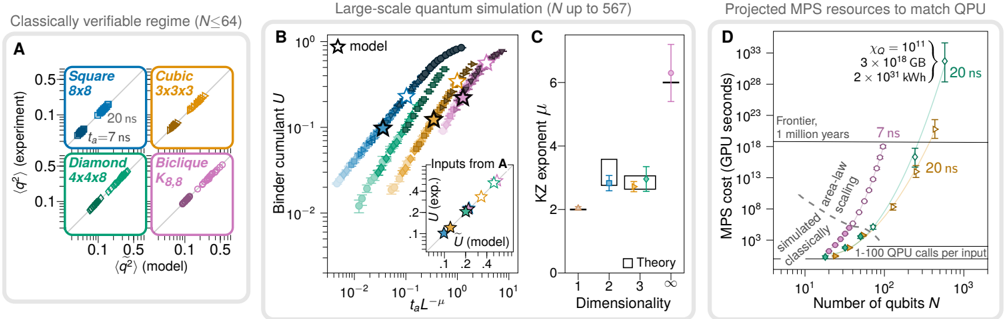
  • Two D-Wave quantum annealing processors, ADV1 and ADV2, produced consistent samples for 2D, 3D, and infinite-dimensional spin-glass quenches; for the largest MPS ground truths, the spin-glass order parameter ⟨q²⟩ had a median deviation of only 1% between quantum and classical simulation.
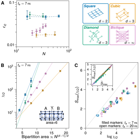
  • MPS required a QPU-equivalent bond dimension χ_Q that grew exponentially with bipartition area, consistent with area-law entanglement scaling; for 3D or biclique lattices the estimated requirement was χ_Q ≃ 10⁷, and for diamond lattices χ_Q ≃ 10¹¹.
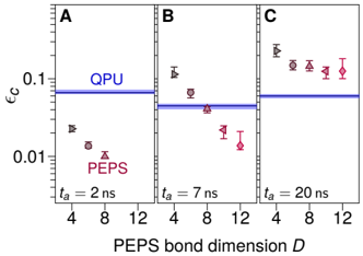
  • PEPS and NQS methods failed to match QPU accuracy even on modest 2D problems at slower quenches: PEPS easily beat QPU error at t_a = 2 ns but at 20 ns all PEPS experiments had higher error than QPU, and NQS could not produce acceptable accuracy beyond the shortest time scales and smallest models.
  • Extrapolated MPS resource estimates indicated that matching QPU quality on the largest problems would take millions of years on the Frontier supercomputer per input, exceed its 700 PB storage, and exceed annual global electricity consumption; extracted KZ exponents, e.g. square 2.83(24), cubic 2.72(16), and biclique 6.3(9), agreed with previous estimates and theory.

Methods

  • The task was to sample from the post-quench state of a time-dependent transverse-field Ising model, H(t) = Γ(t/t_a)H_D + J(t/t_a)H_P, on square, cubic dimer, diamond, and biclique topologies, using two D-Wave processors: ADV1 (5627 qubits) and ADV2 (1222 qubits), both at 12 mK, with each QPU generating at least 1000 samples per second.
  • QPU results were compared with classical approximations to the time-dependent Schrödinger equation: MPS and PEPS tensor networks and NQS simulations; ground truths for small systems came from well-converged MPS simulations on Summit and Frontier, using metrics including correlation error ε_c, classical fidelity F, and QPU-equivalent bond dimension χ_Q.
  • Calibration refinements included flux offsets, anneal offsets, embedding and automorphism averaging, with up to 200 parallel embeddings; the largest diamond input was (12,12,16) with 567 of 576 qubits operable.

Limitations

  • The paper states that direct, nonuniversal verification against ground truth is only possible at small scales; beyond the classically simulable regime, validation relies on universal quantum critical scaling and dynamic finite-size scaling collapse.
  • The paper notes that its resource extrapolation applies to MPS, the only method that matched QPU quality for all considered quench times, and is not an intrinsic lower bound for all classical methods; PEPS and NQS failed at smaller sizes.
  • The paper states that the QPUs were calibrated for the operational regime t_a > 500 ns, while the model quench times studied here required refined time mapping and synchronization corrections; future availability of t_a < 500 ns would make that calibration section unnecessary. The largest diamond lattice permitted 9 defects out of 576 qubits, expected to have no significant impact on algorithmic complexity.

Model-written summary. Check it against the paper before relying on it.

Integrity signals

Registry

Crossref · 10.1126/science.ado6285

Cites

163 of 163 references verified0 citation errors · 0 not checkable

Statistics

Nothing to recompute.

Figures
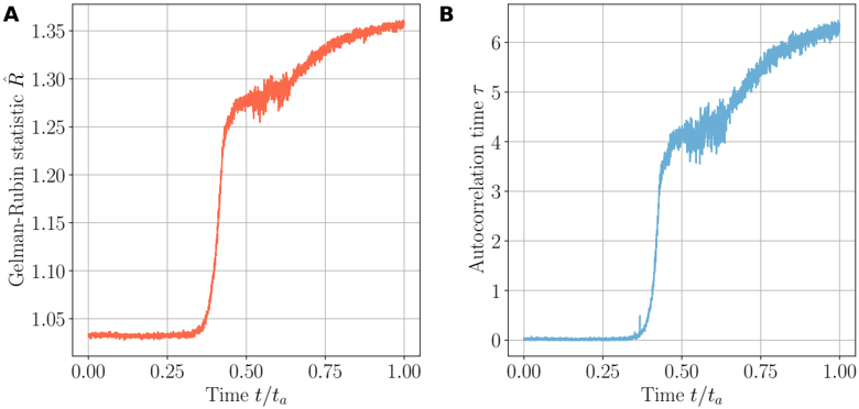
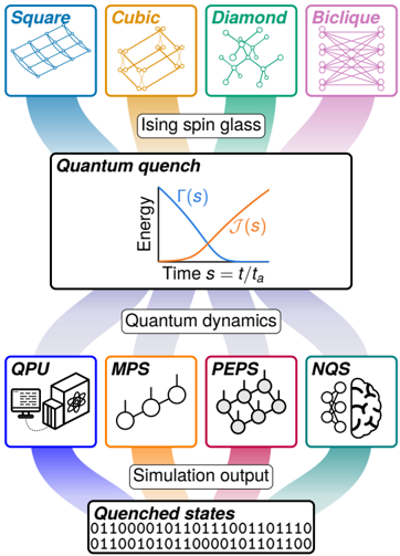
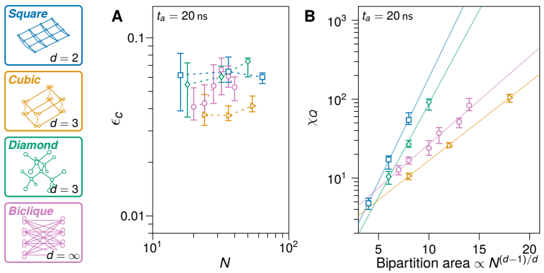
FIG. 1 Sampling post-quench states in Ising spin glasses. Random inputs are generated in topologies of varying dimension. For each input, we consider the task of sampling from the distribution of states following a quantum quench, i.e., rapid change of transverse field Γ( t/t a ) and longitudinal field J ( t/t a ) within time t a . This task is performed using quantum annealing and classical methods based on tensor networks (MPS and PEPS) and neural networks (NQS).
FIG. 1 Sampling post-quench states in Ising spin glasses. Random inputs are generated in topologies of varying dimension. For each input, we consider the task of sampling from the distribution of states following a quantum quench, i.e., rapid change of transverse field Γ( t/t a ) and longitudinal field J ( t/t a ) within time t a . This task is performed using quantum annealing and classical methods based on tensor networks (MPS and PEPS) and neural networks (NQS).CC-BY-NC-ND · From the PDF
Image 2
CC-BY-NC-ND · From the PDF
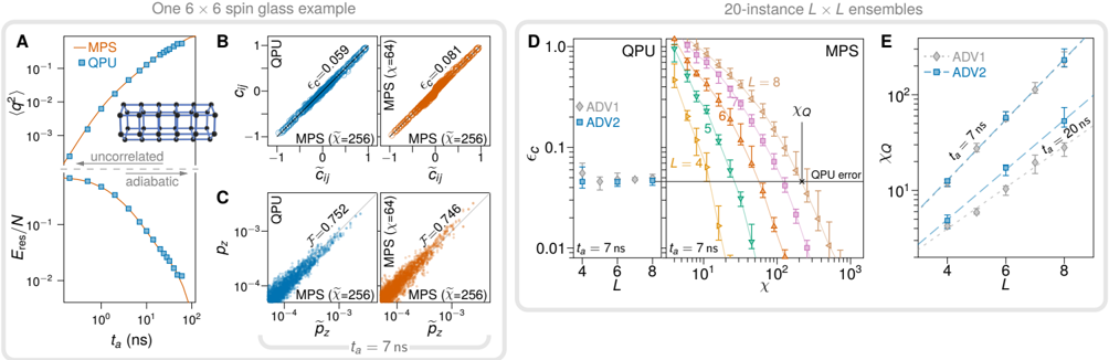
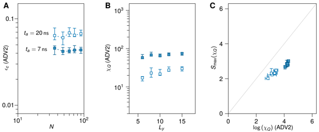
FIG. 2 QPU and MPS on quenched 2D spin glasses. ( A -C ) Data for a typical realization of a 6 × 6 cylindrical spin glass. ( A ) Squared order parameter (top) and residual energy per spin (bottom) data exhibit close agreement between QPU and the ground truth across nearly three decades of t a . In the fast-quench limit t a → 0, correlations and therefore ⟨ q 2 ⟩ are small; in the slow-quench limit t a → ∞ , the system evolves adiabatically and produces classical ground states with vanishing residual energy. Approaching this limit, the problem crosses over into the much easier problem of classical ground-state sampling. ( B ) Spin-spin correlations c ij compared against ground-truth values ˜ c ij for t a =7ns. Left, QPU. Right, MPS at a bond dimension producing output of similar quality. ( C ) Comparison of individual state probabilities for the same simulations as B ; classical fidelities F estimated from 10 6 samples are comparable. ( D -E ) Ensembles of 20 L × L instances (disorder realizations). ( D ) Median correlation error ϵ c remains roughly constant across system sizes for QPU (left), but matching the QPU error level in MPS requires an increasing QPU-equivalent bond dimension χ Q . ( E ) χ Q exhibits exponential growth in L for two quench rates. For t a =20ns, the superior processor, ADV2, shows lower errors, and therefore steeper scaling of χ Q . All error bars represent 95% bootstrap confidence intervals of the ensemble median.
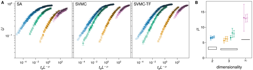
FIG. 2 QPU and MPS on quenched 2D spin glasses. ( A -C ) Data for a typical realization of a 6 × 6 cylindrical spin glass. ( A ) Squared order parameter (top) and residual energy per spin (bottom) data exhibit close agreement between QPU and the ground truth across nearly three decades of t a . In the fast-quench limit t a → 0, correlations and therefore ⟨ q 2 ⟩ are small; in the slow-quench limit t a → ∞ , the system evolves adiabatically and produces classical ground states with vanishing residual energy. Approaching this limit, the problem crosses over into the much easier problem of classical ground-state sampling. ( B ) Spin-spin correlations c ij compared against ground-truth values ˜ c ij for t a =7ns. Left, QPU. Right, MPS at a bond dimension producing output of similar quality. ( C ) Comparison of individual state probabilities for the same simulations as B ; classical fidelities F estimated from 10 6 samples are comparable. ( D -E ) Ensembles of 20 L × L instances (disorder realizations). ( D ) Median correlation error ϵ c remains roughly constant across system sizes for QPU (left), but matching the QPU error level in MPS requires an increasing QPU-equivalent bond dimension χ Q . ( E ) χ Q exhibits exponential growth in L for two quench rates. For t a =20ns, the superior processor, ADV2, shows lower errors, and therefore steeper scaling of χ Q . All error bars represent 95% bootstrap confidence intervals of the ensemble median.CC-BY-NC-ND · From the PDF
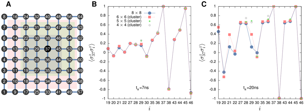
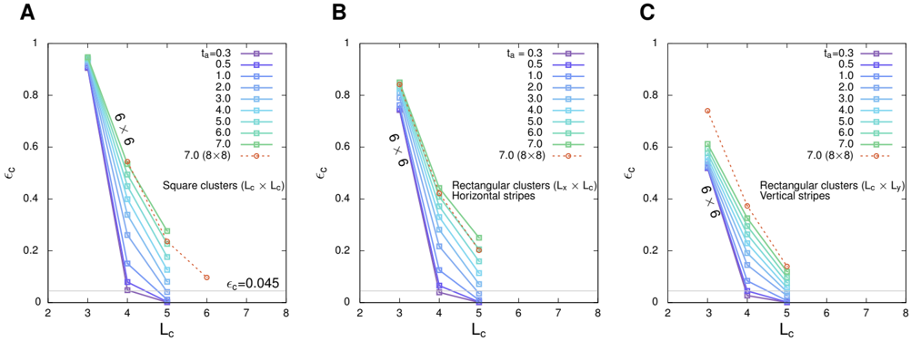
Image 4
CC-BY-NC-ND · From the PDF
FIG. 5 Dynamical scaling and resource estimates for large-scale quantum simulation. ( A ) We compare ⟨ q 2 ⟩ in QPU output and the ground truth for 20 instances of each topology at t a = 7ns and 20 ns, establishing close agreement (median relative error < 1%) for the largest MPS ground truths. ( B ) Using a range of system sizes that we cannot simulate classically, we collapse Binder cumulants U using a dynamic finite-size scaling ansatz, yielding best-fit KZ exponents µ . Curve in collapsed data indicates crossover from power-law (KZ) to system-spanning correlations. Data points are computed from ensembles of 300 to 20,400 simulated spin-glass realizations (collapsed sizes N , indicated by different shades and markers, are 16-324 for square, 54-432 for cubic, 72-567 for diamond, and 32-96 for biclique). Inset: Estimates of U using simulations shown in A for t a = 7ns and 20ns (dark and light stars respectively, also in main plot) show close agreement with the ground truth at simulable sizes, bridging the gap between the classically-simulable and large-scale regimes. ( C ) Extracted KZ exponents for one-, two-, three-, and infinite-dimensional systems agree with previous estimates for the corresponding QPT universality classes. ( D ) Area-law scaling of χ Q (Fig. 4B) allows extrapolation of required classical time based on Nχ 3 Q scaling of MPS methods; all other methods failed at smaller sizes. Filled markers indicate classically-simulated 20-instance ensembles; larger problems are extrapolations.
FIG. 5 Dynamical scaling and resource estimates for large-scale quantum simulation. ( A ) We compare ⟨ q 2 ⟩ in QPU output and the ground truth for 20 instances of each topology at t a = 7ns and 20 ns, establishing close agreement (median relative error < 1%) for the largest MPS ground truths. ( B ) Using a range of system sizes that we cannot simulate classically, we collapse Binder cumulants U using a dynamic finite-size scaling ansatz, yielding best-fit KZ exponents µ . Curve in collapsed data indicates crossover from power-law (KZ) to system-spanning correlations. Data points are computed from ensembles of 300 to 20,400 simulated spin-glass realizations (collapsed sizes N , indicated by different shades and markers, are 16-324 for square, 54-432 for cubic, 72-567 for diamond, and 32-96 for biclique). Inset: Estimates of U using simulations shown in A for t a = 7ns and 20ns (dark and light stars respectively, also in main plot) show close agreement with the ground truth at simulable sizes, bridging the gap between the classically-simulable and large-scale regimes. ( C ) Extracted KZ exponents for one-, two-, three-, and infinite-dimensional systems agree with previous estimates for the corresponding QPT universality classes. ( D ) Area-law scaling of χ Q (Fig. 4B) allows extrapolation of required classical time based on Nχ 3 Q scaling of MPS methods; all other methods failed at smaller sizes. Filled markers indicate classically-simulated 20-instance ensembles; larger problems are extrapolations.CC-BY-NC-ND · From the PDF
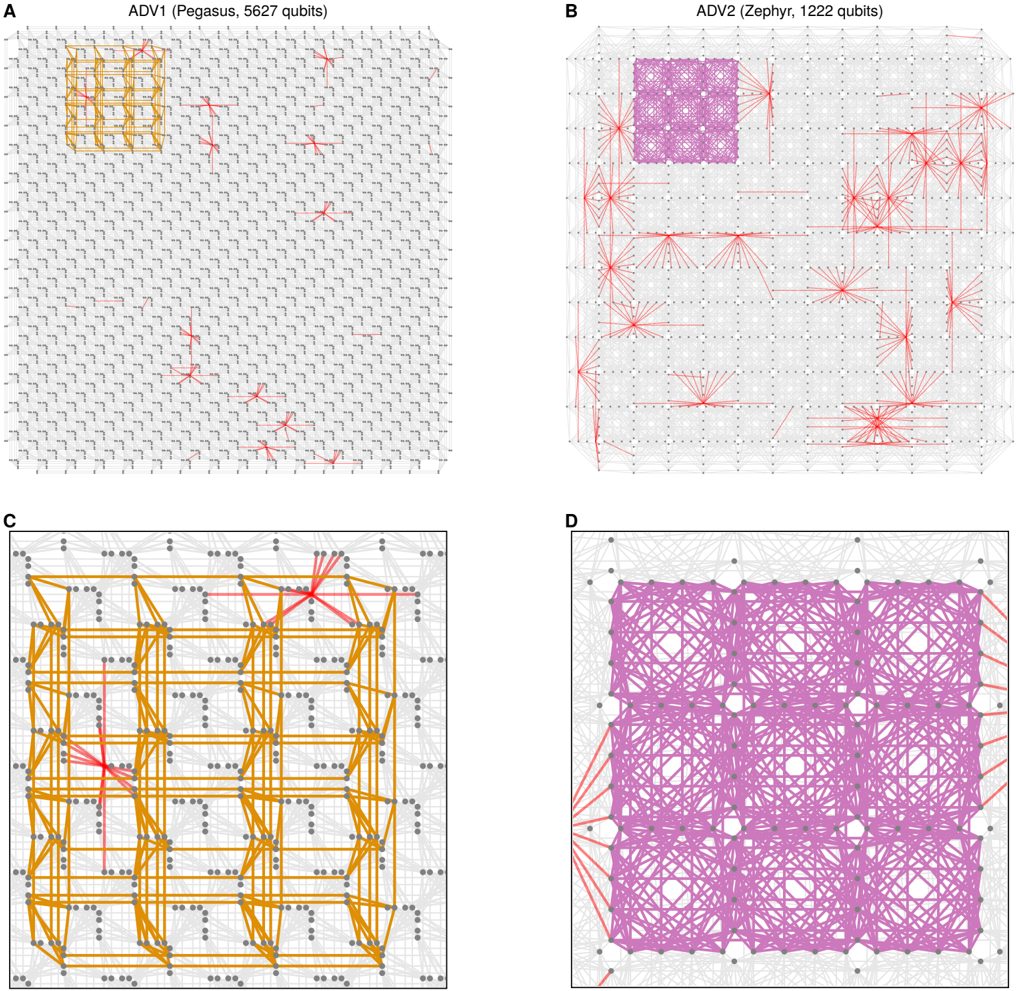
FIG. S1 Qubit connectivity graphs. A , ADV1 and B , ADV2 qubit graphs. Gray points and lines indicate operable qubits and couplers respectively; red points and lines indicate inoperable qubits and couplers. Embeddings of example systems are shown (zoomed, C and D ): cubic dimer, 4 × 4 × 4 dimers in orange, biclique K 24 , 24 with 48 dimers in purple. Diagonal couplings are inter-dimer; horizontal and vertical couplings are intra-dimer.
FIG. S1 Qubit connectivity graphs. A , ADV1 and B , ADV2 qubit graphs. Gray points and lines indicate operable qubits and couplers respectively; red points and lines indicate inoperable qubits and couplers. Embeddings of example systems are shown (zoomed, C and D ): cubic dimer, 4 × 4 × 4 dimers in orange, biclique K 24 , 24 with 48 dimers in purple. Diagonal couplings are inter-dimer; horizontal and vertical couplings are intra-dimer.CC-BY-NC-ND · From the PDF
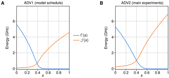
FIG. S2 Annealing schedules for ADV1 and ADV2. A and B show effective TFIM schedules for Advantage and Advantage2 systems, respectively. ADV1 annealing schedule is used to characterize the modeled quench, but ADV2 is used for main measurements, since the Advantage2 processor has lower noise and higher energy scale. The annealing parameter s is a normalized time: s = t/t a .
FIG. S2 Annealing schedules for ADV1 and ADV2. A and B show effective TFIM schedules for Advantage and Advantage2 systems, respectively. ADV1 annealing schedule is used to characterize the modeled quench, but ADV2 is used for main measurements, since the Advantage2 processor has lower noise and higher energy scale. The annealing parameter s is a normalized time: s = t/t a .CC-BY-NC-ND · From the PDF
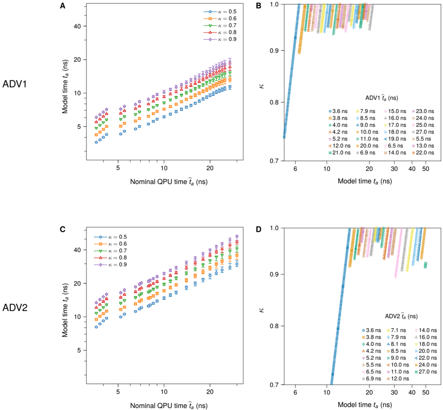
FIG. S3 Calibrating QPU parameters by quench time for ADV1 (top) and ADV2 (bottom) QPUs. A , C , effective model quench time t a is calculated for a range of energy scales κ and nominal quench times ˆ t a (legends); t a is taken as the median effective quench rate (matching ⟨ q 2 ⟩ ) over a 4 × 6 2D spin glass ensemble. B , D , for each t a we choose an appropriate ˆ t a and determine the appropriate κ based on a power-law fit in κ based on the data shown in the left-hand panels.
FIG. S3 Calibrating QPU parameters by quench time for ADV1 (top) and ADV2 (bottom) QPUs. A , C , effective model quench time t a is calculated for a range of energy scales κ and nominal quench times ˆ t a (legends); t a is taken as the median effective quench rate (matching ⟨ q 2 ⟩ ) over a 4 × 6 2D spin glass ensemble. B , D , for each t a we choose an appropriate ˆ t a and determine the appropriate κ based on a power-law fit in κ based on the data shown in the left-hand panels.CC-BY-NC-ND · From the PDF
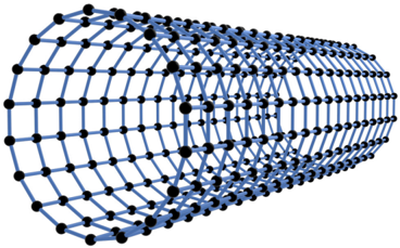
FIG. S4 Square lattice. Largest cylinder embedded on ADV2, 18 × 18, shown.
FIG. S4 Square lattice. Largest cylinder embedded on ADV2, 18 × 18, shown.CC-BY-NC-ND · From the PDF
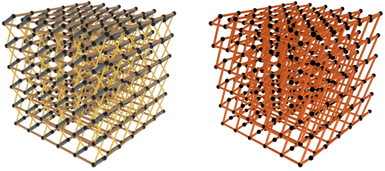
FIG. S5 Cubic dimer and no-dimer lattices. Left, cubic dimer, and right, cubic no-dimer lattices with ( L x , L y , L z ) = (6 , 6 , 6) on 424 qubits. In cubic dimer problems, thick gray lines indicate dimer couplings ( J = -2), dark lines indicate x - and y -dimension couplings, and light yellow lines indicate z -dimension couplings, in which a coupling term is distributed equally between two couplers joining two dimers. In cubic no-dimer inputs (right), all couplers are drawn from the same distribution, and half of the z -couplings from the cubic dimer connectivity are discarded. The disordered 'no-dimer' couplings prevent the spins from being paired into approximately two-level objects. Periodic couplings between top and bottom not shown.
FIG. S5 Cubic dimer and no-dimer lattices. Left, cubic dimer, and right, cubic no-dimer lattices with ( L x , L y , L z ) = (6 , 6 , 6) on 424 qubits. In cubic dimer problems, thick gray lines indicate dimer couplings ( J = -2), dark lines indicate x - and y -dimension couplings, and light yellow lines indicate z -dimension couplings, in which a coupling term is distributed equally between two couplers joining two dimers. In cubic no-dimer inputs (right), all couplers are drawn from the same distribution, and half of the z -couplings from the cubic dimer connectivity are discarded. The disordered 'no-dimer' couplings prevent the spins from being paired into approximately two-level objects. Periodic couplings between top and bottom not shown.CC-BY-NC-ND · From the PDF
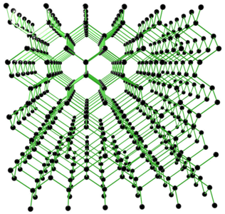
FIG. S6 Diamond lattice. The largest input studied in this work is a diamond lattice with dimensional parameters (12 , 12 , 16), in which 567 of 576 qubits (98.4%) are operable. Inoperable qubits not shown. Periodic couplings between top and bottom not shown.
FIG. S6 Diamond lattice. The largest input studied in this work is a diamond lattice with dimensional parameters (12 , 12 , 16), in which 567 of 576 qubits (98.4%) are operable. Inoperable qubits not shown. Periodic couplings between top and bottom not shown.CC-BY-NC-ND · From the PDF
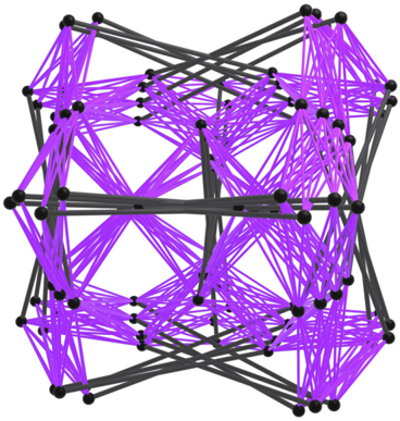
FIG. S7 Biclique lattice. Shown is a K 24 , 24 topology on 96 spins, where gray lines indicate J = -2 coupled dimers, and purple lines indicate inter-dimer couplings, forming a complete bipartite structure.
FIG. S7 Biclique lattice. Shown is a K 24 , 24 topology on 96 spins, where gray lines indicate J = -2 coupled dimers, and purple lines indicate inter-dimer couplings, forming a complete bipartite structure.CC-BY-NC-ND · From the PDF
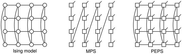
FIG. S8 MPS and PEPS for a small cylindrical TFIM. A 4 × 4 cylindrical transverse-field Ising model may be represented diagrammatically with spins or qubits depicted by circles and couplers depicted by lines (left). To represent a quantum state associated with such a lattice we may use a tensor network (MPS or PEPS). The above diagrams depict contracted networks for purposes of amplitude calculation, as in Eq. (S1). Tensors are represented by squares, lines adjoining two tensors imply a contraction, and free lines depict unsummed indices (in this example, the qubit states). In an MPS (center), the tensors form a path with three indices (lines) per tensor (except on the first and last tensor where there are two), one index or line being of dimension 2 in the depicted case (matching the state-space size of a qubit). In our canonical ordering on a square lattice the tensor contraction circles around the lattice in the periodic dimension, minimizing pathwidth on the target TFIM. Local entanglement is captured indirectly through paths with longer-range connections, but contraction is efficient. In a PEPS (right), one dimension (bond) can be assigned for each non-zero coupling in the TFIM, capturing local full entanglement, but exact contraction is not efficient. In practice, tensor contractions for purposes of time evolution and estimation can be performed iteratively over local subsets, or effective approximate tensor environments, avoiding creation of large objects (many unpaired dimensions).
FIG. S8 MPS and PEPS for a small cylindrical TFIM. A 4 × 4 cylindrical transverse-field Ising model may be represented diagrammatically with spins or qubits depicted by circles and couplers depicted by lines (left). To represent a quantum state associated with such a lattice we may use a tensor network (MPS or PEPS). The above diagrams depict contracted networks for purposes of amplitude calculation, as in Eq. (S1). Tensors are represented by squares, lines adjoining two tensors imply a contraction, and free lines depict unsummed indices (in this example, the qubit states). In an MPS (center), the tensors form a path with three indices (lines) per tensor (except on the first and last tensor where there are two), one index or line being of dimension 2 in the depicted case (matching the state-space size of a qubit). In our canonical ordering on a square lattice the tensor contraction circles around the lattice in the periodic dimension, minimizing pathwidth on the target TFIM. Local entanglement is captured indirectly through paths with longer-range connections, but contraction is efficient. In a PEPS (right), one dimension (bond) can be assigned for each non-zero coupling in the TFIM, capturing local full entanglement, but exact contraction is not efficient. In practice, tensor contractions for purposes of time evolution and estimation can be performed iteratively over local subsets, or effective approximate tensor environments, avoiding creation of large objects (many unpaired dimensions).CC-BY-NC-ND · From the PDF
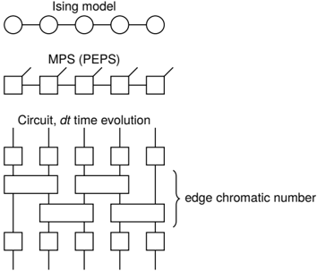
FIG. S9 A PEPS (circuit-model equivalent) representing a 2nd-order Trotterized approximation to time evolution of duration dt . Repeated action of a dt -operator on a PEPS enables a discretized simulation of dynamics with error controlled by dt . The dt operator can be decomposed into 2+ κ layers of rank-2 unitaries (gates), where κ is the edge chromatic number of the lattice being simulated ( κ = 2 = site connectivity for the case of a 1D chain shown). 2-site operators are exp( -i 2 πdt J ( t/t a ) J ij σ z i σ z j ) and single-site operators are exp( -iπdt Γ( t/t a ) σ x i ). The depth of 2-site operators is controlled by κ , and the total number of 2-gates matches the number of edges in the target lattice. To compress the circuit, 1-site operators between time steps can be combined. With care in the order of operations (to ensure 2nd-order Trotterization error), depth can be reduced to κ per unit dt by use of 2-site (rank 4) gates of the form exp ( -i 2 πdt [ J ( t/t a ) J ij σ z i σ z j -Γ( t/t a )( σ x i k i + σ x j k j )] ) , k ∗ being site connectivity, eliminating the need for 1-site gates.
FIG. S9 A PEPS (circuit-model equivalent) representing a 2nd-order Trotterized approximation to time evolution of duration dt . Repeated action of a dt -operator on a PEPS enables a discretized simulation of dynamics with error controlled by dt . The dt operator can be decomposed into 2+ κ layers of rank-2 unitaries (gates), where κ is the edge chromatic number of the lattice being simulated ( κ = 2 = site connectivity for the case of a 1D chain shown). 2-site operators are exp( -i 2 πdt J ( t/t a ) J ij σ z i σ z j ) and single-site operators are exp( -iπdt Γ( t/t a ) σ x i ). The depth of 2-site operators is controlled by κ , and the total number of 2-gates matches the number of edges in the target lattice. To compress the circuit, 1-site operators between time steps can be combined. With care in the order of operations (to ensure 2nd-order Trotterization error), depth can be reduced to κ per unit dt by use of 2-site (rank 4) gates of the form exp ( -i 2 πdt [ J ( t/t a ) J ij σ z i σ z j -Γ( t/t a )( σ x i k i + σ x j k j )] ) , k ∗ being site connectivity, eliminating the need for 1-site gates.CC-BY-NC-ND · From the PDF
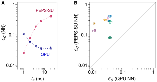
FIG. S10 SU (evolution) plus SO (correlation estimation) versus QPU. ( A ) Ensemble-median 8 × 8 square-lattice (high-precision) correlation error, with numerator and denominator taken only over nearest-neighbor pairs, for SU and QPU. ( B ) Nearest-neighbor correlation error for high-precision square (8 × 8), cubic (3 × 3 × 3), diamond (4 × 4 × 8), and biclique ( K 6 , 6 ) ensembles at t a = 7ns (colored markers) and 20 ns (white markers). PEPS SU+SO errors are smallest on shorter time scales and in models with fewer short loops (like the diamond ensemble), as expected.
FIG. S10 SU (evolution) plus SO (correlation estimation) versus QPU. ( A ) Ensemble-median 8 × 8 square-lattice (high-precision) correlation error, with numerator and denominator taken only over nearest-neighbor pairs, for SU and QPU. ( B ) Nearest-neighbor correlation error for high-precision square (8 × 8), cubic (3 × 3 × 3), diamond (4 × 4 × 8), and biclique ( K 6 , 6 ) ensembles at t a = 7ns (colored markers) and 20 ns (white markers). PEPS SU+SO errors are smallest on shorter time scales and in models with fewer short loops (like the diamond ensemble), as expected.CC-BY-NC-ND · From the PDF
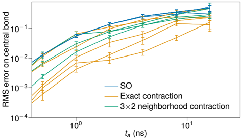
FIG. S11 Absolute correlation error on the (unique) central bond in an open-boundary 3 × 4 J = ± 1 square lattice as a function of quench time. Exact diagonalization methods are applicable at this scale. We present a root mean square error on SU dynamics with respect to 17 disorder realizations. Three different contraction methods for calculation of observables are used, indicated by color, and are combined with SU at various bond dimensions: SO( D = 2 , . . . , 6), 3 × 2 neighbor contraction ( D = 2 , . . . , 4), and exact contraction( D = 2 , . . . , 6). As simulation time approaches zero, all methods approach zero error for bond dimension ≥ 2. At the shortest time shown, error decreases monotonically with bond dimension for all methods. For time ≪ 1 ns all methods converge to zero error at small bond dimension. Approaching the short-time limit, errors go to zero much quicker (in absolute terms shown, and also relative to c ij ), and SO is sufficient. At intermediate time scales estimation quality improves both as a function of neighborhood scale and bond dimension (albeit SO has a very weak dependence on bond dimension). For time ≳ 4 ns all methods approach larger errors, and without a monotonic dependence of error on bond dimension and neighborhood size. Even with no error in observable calculations we see the systematic errors at experimental time scales-larger problems with additional loops can be anticipated to have larger systematic errors, explaining the trends in Figure S10.
FIG. S11 Absolute correlation error on the (unique) central bond in an open-boundary 3 × 4 J = ± 1 square lattice as a function of quench time. Exact diagonalization methods are applicable at this scale. We present a root mean square error on SU dynamics with respect to 17 disorder realizations. Three different contraction methods for calculation of observables are used, indicated by color, and are combined with SU at various bond dimensions: SO( D = 2 , . . . , 6), 3 × 2 neighbor contraction ( D = 2 , . . . , 4), and exact contraction( D = 2 , . . . , 6). As simulation time approaches zero, all methods approach zero error for bond dimension ≥ 2. At the shortest time shown, error decreases monotonically with bond dimension for all methods. For time ≪ 1 ns all methods converge to zero error at small bond dimension. Approaching the short-time limit, errors go to zero much quicker (in absolute terms shown, and also relative to c ij ), and SO is sufficient. At intermediate time scales estimation quality improves both as a function of neighborhood scale and bond dimension (albeit SO has a very weak dependence on bond dimension). For time ≳ 4 ns all methods approach larger errors, and without a monotonic dependence of error on bond dimension and neighborhood size. Even with no error in observable calculations we see the systematic errors at experimental time scales-larger problems with additional loops can be anticipated to have larger systematic errors, explaining the trends in Figure S10.CC-BY-NC-ND · From the PDF
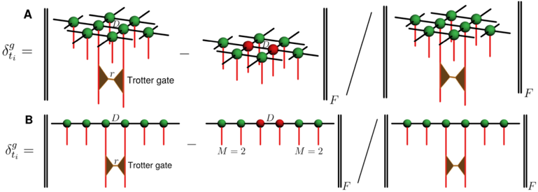
FIG. S12 Optimizing bond dimension truncation in 2D PEPS and non-canonical 1D MPS. In A , for non-canonical PEPS in 2D, the two central tensors are applied with a Trotter gate g with SVD rank r = 2. When the gate tensors are absorbed into the central ones, the bond dimension increases from D to Dr . It is truncated back to D by approximating the central tensors with a pair of new tensors with bond dimension D . The new tensors minimize the Frobenius norm δ g t i of the relative difference between the left and the right diagram, where t i index time steps of the Trotterized evolution. Here, in addition to the two central sites, the 2D cluster includes their six nearest neighbor sites. The total cluster size during such NTU algorithm 96 update is 8 sites. In B , we consider a non-canonical MPS in 1D. Here, in addition to the two central sites, the diagrams include M = 2 sites to the left and M = 2 sites to the right. A total cluster size is 2 + 2 M sites.
FIG. S12 Optimizing bond dimension truncation in 2D PEPS and non-canonical 1D MPS. In A , for non-canonical PEPS in 2D, the two central tensors are applied with a Trotter gate g with SVD rank r = 2. When the gate tensors are absorbed into the central ones, the bond dimension increases from D to Dr . It is truncated back to D by approximating the central tensors with a pair of new tensors with bond dimension D . The new tensors minimize the Frobenius norm δ g t i of the relative difference between the left and the right diagram, where t i index time steps of the Trotterized evolution. Here, in addition to the two central sites, the 2D cluster includes their six nearest neighbor sites. The total cluster size during such NTU algorithm 96 update is 8 sites. In B , we consider a non-canonical MPS in 1D. Here, in addition to the two central sites, the diagrams include M = 2 sites to the left and M = 2 sites to the right. A total cluster size is 2 + 2 M sites.CC-BY-NC-ND · From the PDF
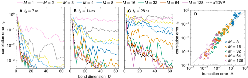
FIG. S13 Correlation and truncation errors in non-canonical MPS. In A , B , and C , we show the correlation error, ϵ c in Eq. (4), as a function of the bond dimension D for annealing times t a = 7, 14, and 28 ns, respectively, for a range of cluster sizes M . For each t a , the function ϵ c ( D ) saturates above a critical value of M . We also show the results of an uniform TDVP (uTDVP) simulations with one-site unit cell 111 , which roughly coincide with the results for the largest clusters in the presented range of parameters. In D , we plot the correlation error as a function of the truncation error ∆ = max ( ∆ AB , ∆ BA ) , according to Eq. (S4). The two are roughly linearly correlated. The correlation error is an order of magnitude lower than the truncation error-the dashed line indicating ∆ / 10 is a guide to the eye. In this panel, t a = 28ns and D = 4 , . . . , 60.
FIG. S13 Correlation and truncation errors in non-canonical MPS. In A , B , and C , we show the correlation error, ϵ c in Eq. (4), as a function of the bond dimension D for annealing times t a = 7, 14, and 28 ns, respectively, for a range of cluster sizes M . For each t a , the function ϵ c ( D ) saturates above a critical value of M . We also show the results of an uniform TDVP (uTDVP) simulations with one-site unit cell 111 , which roughly coincide with the results for the largest clusters in the presented range of parameters. In D , we plot the correlation error as a function of the truncation error ∆ = max ( ∆ AB , ∆ BA ) , according to Eq. (S4). The two are roughly linearly correlated. The correlation error is an order of magnitude lower than the truncation error-the dashed line indicating ∆ / 10 is a guide to the eye. In this panel, t a = 28ns and D = 4 , . . . , 60.CC-BY-NC-ND · From the PDF
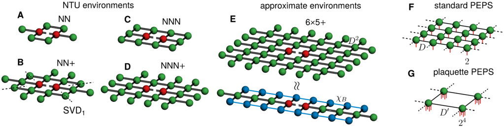
FIG. S14 2D PEPS: environments for truncating enlarged bonds in time-evolution simulations. The two-layer diagrams correspond to the calculation of the Frobenius norms depicted in Fig. S12A. In panel A , we show the neighborhood tensor update environment and, in B -D , its direct extensions that are contracted numerically exactly. In B , SVD 1 indicates a product approximation, where we retain a single leading singular value for tensor decomposition along black dashed cuts. Larger environments, such as the one in E , require approximate contraction, which, however, might disrupt the positivity of the depicted bond metric. Here, to that end, we employ boundary MPS. In F , we indicate a standard PEPS representation with one tensor per spin and, in G , a plaquette PEPS with one tensor for four spins. While a 2 × 2 plaquette of a standard PEPS with bond dimension D can be contracted into a single plaquette PEPS tensor of dimension D 2 , such bonds might not be used optimally. Indeed, we observe that a larger effective environment in plaquette PEPS might result in the compression of the required bond dimension, D ′ < D 2 , for reaching similar accuracy.
FIG. S14 2D PEPS: environments for truncating enlarged bonds in time-evolution simulations. The two-layer diagrams correspond to the calculation of the Frobenius norms depicted in Fig. S12A. In panel A , we show the neighborhood tensor update environment and, in B -D , its direct extensions that are contracted numerically exactly. In B , SVD 1 indicates a product approximation, where we retain a single leading singular value for tensor decomposition along black dashed cuts. Larger environments, such as the one in E , require approximate contraction, which, however, might disrupt the positivity of the depicted bond metric. Here, to that end, we employ boundary MPS. In F , we indicate a standard PEPS representation with one tensor per spin and, in G , a plaquette PEPS with one tensor for four spins. While a 2 × 2 plaquette of a standard PEPS with bond dimension D can be contracted into a single plaquette PEPS tensor of dimension D 2 , such bonds might not be used optimally. Indeed, we observe that a larger effective environment in plaquette PEPS might result in the compression of the required bond dimension, D ′ < D 2 , for reaching similar accuracy.CC-BY-NC-ND · From the PDF
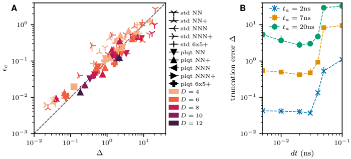
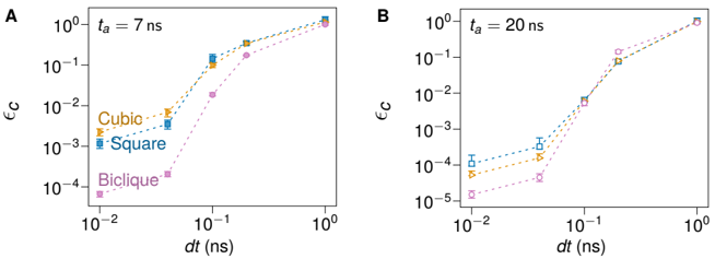
FIG. S15 2D PEPS: Correlation errors vs truncation error. In A, we compare the correlation errors ϵ c with the truncation error in Eq. (S4). The two quantities are roughly linearly correlated for a broad range of simulation parameters, with ϵ c being an order of magnitude smaller than ∆. The dashed line showing ϵ c = ∆ / 10 is a guide for an eye. Each point corresponds to a different PEPS bond dimension (color), the environment used for truncation (symbols, see Fig. S14), annealing time, and coupling precision (the latter two are not distinguished by color nor symbol). Data for 8 × 8 cylindric lattice. In B, we show the convergence of ∆ with dt → 0, where the data are for plaquette PEPS with NN+ environments and D = 10.
FIG. S15 2D PEPS: Correlation errors vs truncation error. In A, we compare the correlation errors ϵ c with the truncation error in Eq. (S4). The two quantities are roughly linearly correlated for a broad range of simulation parameters, with ϵ c being an order of magnitude smaller than ∆. The dashed line showing ϵ c = ∆ / 10 is a guide for an eye. Each point corresponds to a different PEPS bond dimension (color), the environment used for truncation (symbols, see Fig. S14), annealing time, and coupling precision (the latter two are not distinguished by color nor symbol). Data for 8 × 8 cylindric lattice. In B, we show the convergence of ∆ with dt → 0, where the data are for plaquette PEPS with NN+ environments and D = 10.CC-BY-NC-ND · From the PDF
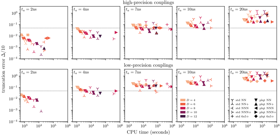
FIG. S16 2D PEPS: errors vs numerical costs. We show estimates of PEPS accuracy, employing truncation errors ∆ / 10, as a function of simulation times for problems defined on 8 × 8 cylinders. Each panel corresponds to a fixed annealing time and type of random couplings (high- or low-precision, see Sec. II). Points in each panel represent PEPS attempts to simulate a given problem for a selection of PEPS bond dimensions and type of environment used in truncation (see Fig. S14). Those plots complement Fig. 3 of the main text, which shows the correlation errors for t a = 2, 7, and 20 ns for high-precision couplings. We see systematic accuracy improvements with the bond dimension for shorter annealing times. This trend systematically stagnates for slower evolutions, where the necessity to employ larger environments becomes apparent. The low-precision couplings prove more challenging for PEPS to simulate than the high-precision. Indeed, energy degeneracies related to discrete J = ± 1 couplings are expected to facilitate entanglement spreading as compared to high-precision inputs, where such degeneracies are much less common. As CPU times, we report simulation wall times executed on a single CPU core.
FIG. S16 2D PEPS: errors vs numerical costs. We show estimates of PEPS accuracy, employing truncation errors ∆ / 10, as a function of simulation times for problems defined on 8 × 8 cylinders. Each panel corresponds to a fixed annealing time and type of random couplings (high- or low-precision, see Sec. II). Points in each panel represent PEPS attempts to simulate a given problem for a selection of PEPS bond dimensions and type of environment used in truncation (see Fig. S14). Those plots complement Fig. 3 of the main text, which shows the correlation errors for t a = 2, 7, and 20 ns for high-precision couplings. We see systematic accuracy improvements with the bond dimension for shorter annealing times. This trend systematically stagnates for slower evolutions, where the necessity to employ larger environments becomes apparent. The low-precision couplings prove more challenging for PEPS to simulate than the high-precision. Indeed, energy degeneracies related to discrete J = ± 1 couplings are expected to facilitate entanglement spreading as compared to high-precision inputs, where such degeneracies are much less common. As CPU times, we report simulation wall times executed on a single CPU core.CC-BY-NC-ND · From the PDF
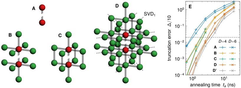
FIG. S17 3D PEPS. The left panel shows four out of five truncation clusters used in 3D PEPS time evolution. The diagrams represent Gramm-Schmidt metric tensors that measure the truncation error. With cluster A the truncation is just an SVD, cluster B includes whole nearest-neighbor tensors (more than the simple update), and C includes vertical bonds between the nearest-neighbor tensors (like the 2D NTU, called 3DNN). Cluster D reaches out to third nearest neighbors but is made tree-like by SVD truncations to just the single leading singular value (SVD 1 ) that are marked by the black dashed cuts. The biggest cluster D' (not shown) is a 5 × 5 × 6 rectangle made tree-like with a few SVD 1 . The right panel, E , shows total truncation error as a function of the annealing time t a for clusters A , B , C , D , D' and bond dimensions D = 4 and 6. Here L = 8, dt = 0 . 01 ns, and the error bars result from averaging over 8 realizations of the random couplings. A dashed line indicates a 2% level of error obtained in QPU simulations for 3D problems with dimers.
FIG. S17 3D PEPS. The left panel shows four out of five truncation clusters used in 3D PEPS time evolution. The diagrams represent Gramm-Schmidt metric tensors that measure the truncation error. With cluster A the truncation is just an SVD, cluster B includes whole nearest-neighbor tensors (more than the simple update), and C includes vertical bonds between the nearest-neighbor tensors (like the 2D NTU, called 3DNN). Cluster D reaches out to third nearest neighbors but is made tree-like by SVD truncations to just the single leading singular value (SVD 1 ) that are marked by the black dashed cuts. The biggest cluster D' (not shown) is a 5 × 5 × 6 rectangle made tree-like with a few SVD 1 . The right panel, E , shows total truncation error as a function of the annealing time t a for clusters A , B , C , D , D' and bond dimensions D = 4 and 6. Here L = 8, dt = 0 . 01 ns, and the error bars result from averaging over 8 realizations of the random couplings. A dashed line indicates a 2% level of error obtained in QPU simulations for 3D problems with dimers.CC-BY-NC-ND · From the PDF
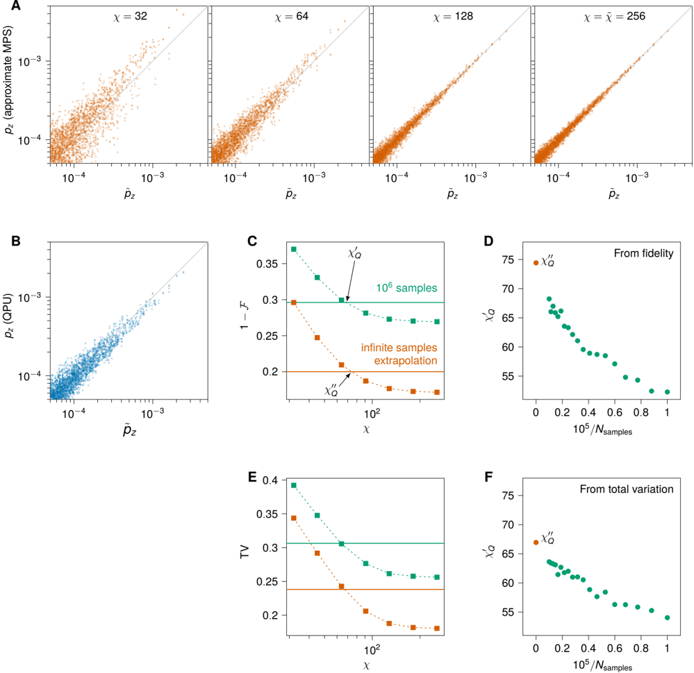
FIG. S18 Estimating QPU-equivalent bond dimension from classical fidelity. ( A ) Fig. 2C (right) is extended, with data for four MPS bond dimensions, up to and including the ground-truth bond dimension ˜ χ , for which only sampling error remains. ( B ) Fig. 2C (left) is shown for comparison, qualitatively similar in spread to χ = 64. ( C ) We can estimate the QPUequivalent bond dimension from F instead of from ϵ c , by using 10 6 samples or by extrapolating to the limit of infinitely many samples drawn. We call these quantities χ ′ Q and χ ′′ Q , similar to the estimate χ Q derived from correlation error. Analogously to χ Q , error (1 -F in this case) is plotted for a range of MPS bond dimensions and the crossing point of QPU error (solid horizontal lines) gives the QPU-equivalent bond dimension. ( D ) χ ′ Q is shown for varying resampled sets of size 10 5 to 10 6 , and plotted against the inverse sample size along with χ ′′ Q . ( E -F ) analysis of D-E is repeated using total variation (TV) in place of 1 -F .
FIG. S18 Estimating QPU-equivalent bond dimension from classical fidelity. ( A ) Fig. 2C (right) is extended, with data for four MPS bond dimensions, up to and including the ground-truth bond dimension ˜ χ , for which only sampling error remains. ( B ) Fig. 2C (left) is shown for comparison, qualitatively similar in spread to χ = 64. ( C ) We can estimate the QPUequivalent bond dimension from F instead of from ϵ c , by using 10 6 samples or by extrapolating to the limit of infinitely many samples drawn. We call these quantities χ ′ Q and χ ′′ Q , similar to the estimate χ Q derived from correlation error. Analogously to χ Q , error (1 -F in this case) is plotted for a range of MPS bond dimensions and the crossing point of QPU error (solid horizontal lines) gives the QPU-equivalent bond dimension. ( D ) χ ′ Q is shown for varying resampled sets of size 10 5 to 10 6 , and plotted against the inverse sample size along with χ ′′ Q . ( E -F ) analysis of D-E is repeated using total variation (TV) in place of 1 -F .CC-BY-NC-ND · From the PDF
FIG. S19 Comparing correlation-based and fidelity-based QPU-equivalent bond dimensions. Shown are χ Q and χ ′′ Q (as in Fig. 2D and Fig. S18C respectively), with χ ′′ Q computed from fidelity (top) and total variation (bottom). At a fixed maximum sample size 10 6 , we expect χ ′′ Q to deviate downwards from χ Q for systems of increasing entropy, since inference requires exponentially many samples.
FIG. S19 Comparing correlation-based and fidelity-based QPU-equivalent bond dimensions. Shown are χ Q and χ ′′ Q (as in Fig. 2D and Fig. S18C respectively), with χ ′′ Q computed from fidelity (top) and total variation (bottom). At a fixed maximum sample size 10 6 , we expect χ ′′ Q to deviate downwards from χ Q for systems of increasing entropy, since inference requires exponentially many samples.CC-BY-NC-ND · From the PDF
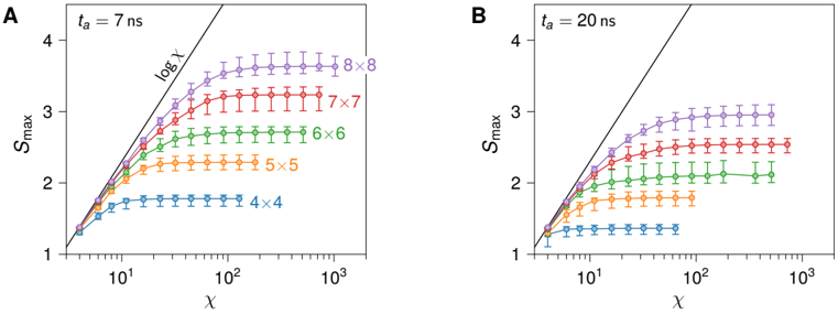
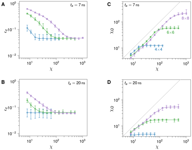
FIG. S20 Convergence of peak entanglement entropy. Entanglement S max grows as a function of MPS bond dimension χ , converging in the χ →∞ limit. A and B show this convergence in 2D models for 7 ns and 20 ns quenches, respectively. The line log( χ ) indicates the upper bound of entanglement that can be expressed in an MPS of bond dimension χ .
FIG. S20 Convergence of peak entanglement entropy. Entanglement S max grows as a function of MPS bond dimension χ , converging in the χ →∞ limit. A and B show this convergence in 2D models for 7 ns and 20 ns quenches, respectively. The line log( χ ) indicates the upper bound of entanglement that can be expressed in an MPS of bond dimension χ .CC-BY-NC-ND · From the PDF
FIG. S21 Convergence of error and equivalent bond dimension as a function of ground-truth bond dimension. As in Fig. S20, we study square lattices at t a = 7ns and t a = 20ns. QPU error ϵ c ( A -B ) and QPU-equivalent bond dimension χ Q ( C -D ) are shown as a function of MPS bond dimension χ . The MPS used for the ground truth must have sufficient bond dimension such that these quantities are converged. Gray lines indicate the upper bound χ Q ≤ χ .
FIG. S21 Convergence of error and equivalent bond dimension as a function of ground-truth bond dimension. As in Fig. S20, we study square lattices at t a = 7ns and t a = 20ns. QPU error ϵ c ( A -B ) and QPU-equivalent bond dimension χ Q ( C -D ) are shown as a function of MPS bond dimension χ . The MPS used for the ground truth must have sufficient bond dimension such that these quantities are converged. Gray lines indicate the upper bound χ Q ≤ χ .CC-BY-NC-ND · From the PDF
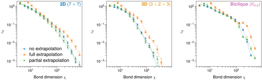
FIG. S22 Effect of extrapolation in MPS bond dimension on correlation errors. MPS experiments of varying χ are evaluated under three types of two-point extrapolation of spin-spin correlations, in terms of their error against a well-converged ground truth with t a = 7ns.
FIG. S22 Effect of extrapolation in MPS bond dimension on correlation errors. MPS experiments of varying χ are evaluated under three types of two-point extrapolation of spin-spin correlations, in terms of their error against a well-converged ground truth with t a = 7ns.CC-BY-NC-ND · From the PDF
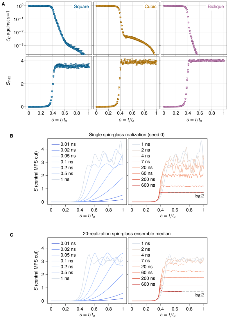
FIG. S23 MPS error from stopping at s < 1 , compared with growth of entanglement entropy. ( A ) (Top) We plot median correlation error of MPS correlations throughout the quench, using a reference ground truth at s = 1. Square (8 × 8, left), cubic (3 × 3 × 3, middle), and biclique ( K 8 , 8 , right) ensembles ( t a = 7ns, χ = 1024) approach the s → 1 limit in varying manner. (Bottom) Growth of ensemble-median S max (maximum over MPS cuts for each instance) saturates when ϵ c is near 0 . 1, higher than QPU error, consistent with Fig. 4C (inset). ( B ) Bipartite entanglement entropy in a single 8 × 8 spin-glass instance, taken across the central MPS cut (32 spins on each side) as a function of s for varying t a . Even t a = 1ns is far slower than the speed-limited regime in which entanglement grows monotonically as a function of s . ( C ) Central-cut entanglement entropy, median over 20 8 × 8 spin-glass instances. All 20 inputs have only two classical ground states, related by spin-flip symmetry, so the ground state as s → 1 is the GHZ state between them, with S = log 2.
FIG. S23 MPS error from stopping at s < 1 , compared with growth of entanglement entropy. ( A ) (Top) We plot median correlation error of MPS correlations throughout the quench, using a reference ground truth at s = 1. Square (8 × 8, left), cubic (3 × 3 × 3, middle), and biclique ( K 8 , 8 , right) ensembles ( t a = 7ns, χ = 1024) approach the s → 1 limit in varying manner. (Bottom) Growth of ensemble-median S max (maximum over MPS cuts for each instance) saturates when ϵ c is near 0 . 1, higher than QPU error, consistent with Fig. 4C (inset). ( B ) Bipartite entanglement entropy in a single 8 × 8 spin-glass instance, taken across the central MPS cut (32 spins on each side) as a function of s for varying t a . Even t a = 1ns is far slower than the speed-limited regime in which entanglement grows monotonically as a function of s . ( C ) Central-cut entanglement entropy, median over 20 8 × 8 spin-glass instances. All 20 inputs have only two classical ground states, related by spin-flip symmetry, so the ground state as s → 1 is the GHZ state between them, with S = log 2.CC-BY-NC-ND · From the PDF
Image 29
CC-BY-NC-ND · From the PDF
Image 30
CC-BY-NC-ND · From the PDF
Image 31
CC-BY-NC-ND · From the PDF
FIG. S27 Monte Carlo convergence statistics for an 8 × 8 instance at 7 ns. (A) Gelman-Rubin statistic ( ˆ R ) plotted versus time 139 . A value of < 1 . 1 indicates that Markov chains are converging 140 . (B) Autocorrelation time ( τ ) of the Markov chain. Longer autocorrelation times mean that more sweeps are required to obtain uncorrelated samples. Both statistics indicate that as we pass through the critical point, the Monte Carlo sampling becomes more difficult, resulting in a higher number of samples required to obtain the correct dynamics.
FIG. S27 Monte Carlo convergence statistics for an 8 × 8 instance at 7 ns. (A) Gelman-Rubin statistic ( ˆ R ) plotted versus time 139 . A value of < 1 . 1 indicates that Markov chains are converging 140 . (B) Autocorrelation time ( τ ) of the Markov chain. Longer autocorrelation times mean that more sweeps are required to obtain uncorrelated samples. Both statistics indicate that as we pass through the critical point, the Monte Carlo sampling becomes more difficult, resulting in a higher number of samples required to obtain the correct dynamics.CC-BY-NC-ND · From the PDF
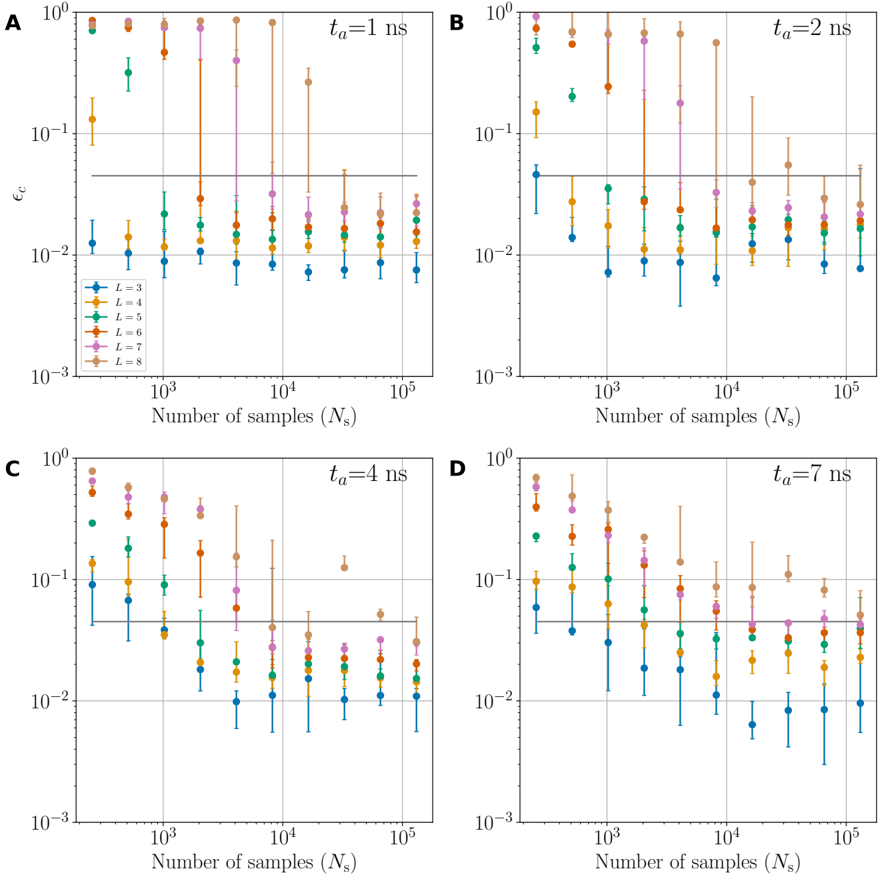
FIG. S28 Average correlation error for a system of size L × L using the cRBM. The correlations are estimated with a total of 10 6 samples (equivalent to QPU). Error bars represent the standard deviation across 5 different disorder realizations. We focus on correlations at s = 0 . 6 due to the smallest correlation error observed at this point (see also Figure S23). Depending on the system size and number of samples N s , we increased the number of GPUs from 1 to 8 and implemented a chunking scheme that splits up the total number of samples into batches. This reduces memory requirements at the expense of increased compute time. ( A-C ) For times up to 4 ns, matching the QPU error is achievable for larger system sizes by increasing N s . ( D ) As system sizes grow, matching the QPU error becomes more challenging. For all time scales, we observe that the error plateaus after reaching a certain sample count.
FIG. S28 Average correlation error for a system of size L × L using the cRBM. The correlations are estimated with a total of 10 6 samples (equivalent to QPU). Error bars represent the standard deviation across 5 different disorder realizations. We focus on correlations at s = 0 . 6 due to the smallest correlation error observed at this point (see also Figure S23). Depending on the system size and number of samples N s , we increased the number of GPUs from 1 to 8 and implemented a chunking scheme that splits up the total number of samples into batches. This reduces memory requirements at the expense of increased compute time. ( A-C ) For times up to 4 ns, matching the QPU error is achievable for larger system sizes by increasing N s . ( D ) As system sizes grow, matching the QPU error becomes more challenging. For all time scales, we observe that the error plateaus after reaching a certain sample count.CC-BY-NC-ND · From the PDF
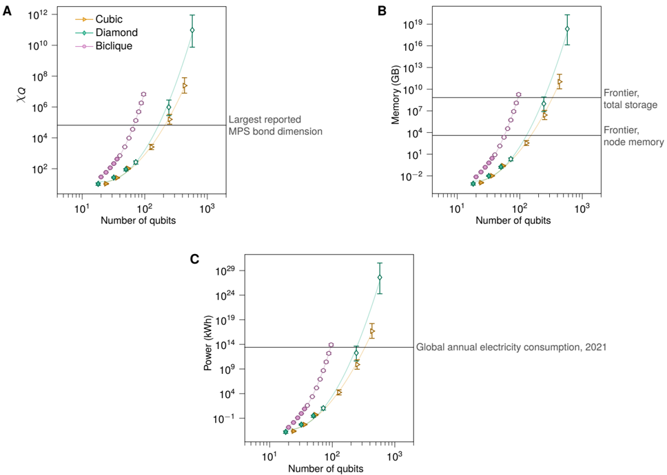
FIG. S29 Resource requirements for MPS to match QPU quality. ( A ) Area-law extrapolation is used to estimate the QPU-equivalent bond dimension χ Q required by MPS methods to achieve QPU-level accuracy. Values far exceed the largest reported MPS bond dimension to date 81 . ( B ) Dominant scaling of memory is ∝ Nχ 2 Q ; assuming this form we compute MPS memory requirements, which exceed both Frontier node flash memory (4 TB) and total storage of the Frontier filesystem (700 PB). ( C ) Power, like computation time, scales ∝ t a Nχ 3 Q . Here, GPU-time requirements (Fig. 5D) are converted to power requirements based on 300 W draw of an Nvidia Tesla V100. These requirements far exceed the total global electricity consumption throughout human history. All plots use t a = 7ns for biclique problems and t a = 20ns for diamond and cubic problems.
FIG. S29 Resource requirements for MPS to match QPU quality. ( A ) Area-law extrapolation is used to estimate the QPU-equivalent bond dimension χ Q required by MPS methods to achieve QPU-level accuracy. Values far exceed the largest reported MPS bond dimension to date 81 . ( B ) Dominant scaling of memory is ∝ Nχ 2 Q ; assuming this form we compute MPS memory requirements, which exceed both Frontier node flash memory (4 TB) and total storage of the Frontier filesystem (700 PB). ( C ) Power, like computation time, scales ∝ t a Nχ 3 Q . Here, GPU-time requirements (Fig. 5D) are converted to power requirements based on 300 W draw of an Nvidia Tesla V100. These requirements far exceed the total global electricity consumption throughout human history. All plots use t a = 7ns for biclique problems and t a = 20ns for diamond and cubic problems.CC-BY-NC-ND · From the PDF
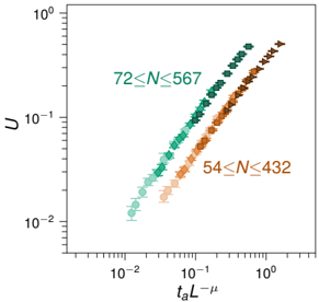
FIG. S30 Dynamic finite-size scaling collapse for diamond and cubic no-dimer instances. Curves of collapsed Binder cumulant U for diamond (green) and cubic no-dimer instances (orange).
FIG. S30 Dynamic finite-size scaling collapse for diamond and cubic no-dimer instances. Curves of collapsed Binder cumulant U for diamond (green) and cubic no-dimer instances (orange).CC-BY-NC-ND · From the PDF
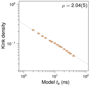
FIG. S31 Kink density in pure 1D quantum Ising chain. Density of kinks (frustrated bonds) are shown as a function of t a for a pure antiferromagnetic 1D chain with length L = 512. Assuming a kink density proportional to t -1 /µ a yields an estimate µ = 2 . 04(5), in agreement with theory.
FIG. S31 Kink density in pure 1D quantum Ising chain. Density of kinks (frustrated bonds) are shown as a function of t a for a pure antiferromagnetic 1D chain with length L = 512. Assuming a kink density proportional to t -1 /µ a yields an estimate µ = 2 . 04(5), in agreement with theory.CC-BY-NC-ND · From the PDF
FIG. S32 Dynamic finite-size scaling for Monte Carlo dynamics. ( A ) Binder cumulant collapses for high-precision instances as in Fig. 5B for SA, SVMC, and SVMC-TF dynamics. Blue, yellow, green, and purple data are from square, cubic, diamond, and biclique lattices respectively. ( B ) Extracted KZ exponents µ , with quantum estimates indicated in black. For biclique problems we use the quantum upper-critical dimension of 8 rather than the classical value of 6, since we are testing consistency with quantum dynamics. Dark, medium, and white shaded markers indicate SA, SVMC, and SVMC-TF values respectively. Estimates are taken from high-precision instances only.
FIG. S32 Dynamic finite-size scaling for Monte Carlo dynamics. ( A ) Binder cumulant collapses for high-precision instances as in Fig. 5B for SA, SVMC, and SVMC-TF dynamics. Blue, yellow, green, and purple data are from square, cubic, diamond, and biclique lattices respectively. ( B ) Extracted KZ exponents µ , with quantum estimates indicated in black. For biclique problems we use the quantum upper-critical dimension of 8 rather than the classical value of 6, since we are testing consistency with quantum dynamics. Dark, medium, and white shaded markers indicate SA, SVMC, and SVMC-TF values respectively. Estimates are taken from high-precision instances only.CC-BY-NC-ND · From the PDF
FIG. S33 Short-range correlations . Panel A shows the 6 × 6 (red), 5 × 5 (green), 4 × 4 (gray) clusters embedded in the 8 × 8 system, around site number 37. Correlations with respect to site=37, c 37 ,i , are shown for various cluster sizes in B ( t a = 7ns) and C (20 ns). Correlations are only shown with respect to the central sites compatible with all clusters.
FIG. S33 Short-range correlations . Panel A shows the 6 × 6 (red), 5 × 5 (green), 4 × 4 (gray) clusters embedded in the 8 × 8 system, around site number 37. Correlations with respect to site=37, c 37 ,i , are shown for various cluster sizes in B ( t a = 7ns) and C (20 ns). Correlations are only shown with respect to the central sites compatible with all clusters.CC-BY-NC-ND · From the PDF
FIG. S34 Correlation matrix error . Panels A , B , and C show ϵ c for various t a as a function of cluster size using the square cluster, open stripes, and periodic stripes, respectively. All results are for the full system of 6 × 6, except red dashed lines, which depict the ϵ c of TCA on the 8 × 8 system. Legend values are provided in nanoseconds.
FIG. S34 Correlation matrix error . Panels A , B , and C show ϵ c for various t a as a function of cluster size using the square cluster, open stripes, and periodic stripes, respectively. All results are for the full system of 6 × 6, except red dashed lines, which depict the ϵ c of TCA on the 8 × 8 system. Legend values are provided in nanoseconds.CC-BY-NC-ND · From the PDF
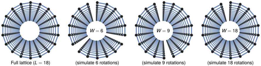
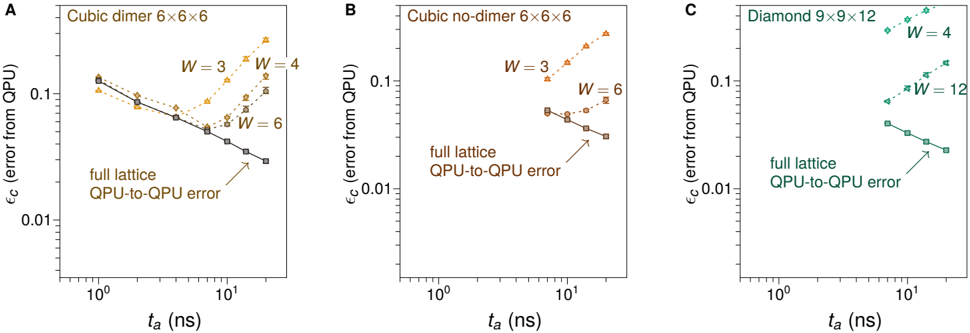
FIG. S35 Rotating clusters in 2D. For fast quenches, where final states have only short-ranged correlations, spoofing approaches can be based on simulating cheaper clusters-with one dimension having width W smaller than the linear system size L -within the full lattice, then recombining output. We evaluate this approach for square, cubic, and cubic no-dimer lattices. Shown are examples of cluster shapes simulated in an effort to spoof 18 × 18 square lattice results.
FIG. S35 Rotating clusters in 2D. For fast quenches, where final states have only short-ranged correlations, spoofing approaches can be based on simulating cheaper clusters-with one dimension having width W smaller than the linear system size L -within the full lattice, then recombining output. We evaluate this approach for square, cubic, and cubic no-dimer lattices. Shown are examples of cluster shapes simulated in an effort to spoof 18 × 18 square lattice results.CC-BY-NC-ND · From the PDF
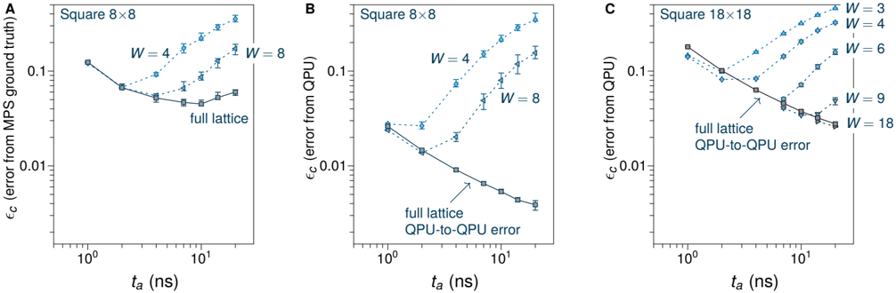
FIG. S36 Error from rotating clusters in 2D. ( A ) QPU simulation is performed for 8 × 8 square lattices, on the full lattice (solid line) and using a rotating cluster approximation (dashed lines). We can compute MPS ground truths and measure ϵ c directly for varying values of W . For W = 8, where each cluster is the same size as the full lattice, significant deviations from the full-lattice error level are seen for t a > 4 ns. ( B ) Here, error for the same experiments as in A is computed not from a ground truth, but from a full-lattice quantum simulation. An independently-run full-lattice simulation gives a noise floor marked by a solid line and square markers (which can be beaten due to averaging of clusters and smoothing of statistical noise). Error against QA appears to lower-bound error against ground truth. ( C ) 18 × 18 system for which ground truth cannot be computed. At W = 18, ϵ c is indistinguishable from the full lattice simulation even for t a = 20ns.
FIG. S36 Error from rotating clusters in 2D. ( A ) QPU simulation is performed for 8 × 8 square lattices, on the full lattice (solid line) and using a rotating cluster approximation (dashed lines). We can compute MPS ground truths and measure ϵ c directly for varying values of W . For W = 8, where each cluster is the same size as the full lattice, significant deviations from the full-lattice error level are seen for t a > 4 ns. ( B ) Here, error for the same experiments as in A is computed not from a ground truth, but from a full-lattice quantum simulation. An independently-run full-lattice simulation gives a noise floor marked by a solid line and square markers (which can be beaten due to averaging of clusters and smoothing of statistical noise). Error against QA appears to lower-bound error against ground truth. ( C ) 18 × 18 system for which ground truth cannot be computed. At W = 18, ϵ c is indistinguishable from the full lattice simulation even for t a = 20ns.CC-BY-NC-ND · From the PDF
FIG. S37 Error from rotating clusters in 3D. ( A ) Cubic dimer and ( B ) cubic no-dimer at the largest simulated size (432 qubits), and ( C ) diamond inputs at the largest defect-free simulated size (243 qubits). As with 2D systems, correlations from full-lattice simulation are compared against composed correlations from multiple simulations with varying cluster size. For W = L , the deviation of ϵ c from the statistical floor (solid lines) indicates that a moving cluster containing all qubits, but with a single row of couplers deleted, is insufficient to capture correlations in the system for all three lattice types beyond short time scales.
FIG. S37 Error from rotating clusters in 3D. ( A ) Cubic dimer and ( B ) cubic no-dimer at the largest simulated size (432 qubits), and ( C ) diamond inputs at the largest defect-free simulated size (243 qubits). As with 2D systems, correlations from full-lattice simulation are compared against composed correlations from multiple simulations with varying cluster size. For W = L , the deviation of ϵ c from the statistical floor (solid lines) indicates that a moving cluster containing all qubits, but with a single row of couplers deleted, is insufficient to capture correlations in the system for all three lattice types beyond short time scales.CC-BY-NC-ND · From the PDF
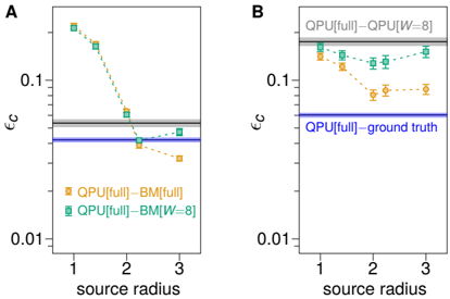
FIG. S38 Error by extrapolation from local correlation estimates on 8 × 8 cylinders. ( A ) t a = 7ns and ( B ) t a = 20ns. The divergence of the QPU from the ground-truth distribution is shown by the blue horizontal line. If the QPU distribution can be reconstructed from a rotating-cluster approximation with similar accuracy, we anticipate an equal-scale clustering approach can also be used for ground-truth estimation, as verified at smaller scale. Correlations on 8 × 8 cylinder models can be estimated by rotating clusters with one cut (Fig. S35 right); correlations are more accurate furthest from the cut. For each correlation, we can select a rotating cluster with the cut maximally separated from the site coordinates, yielding an error shown by the black horizontal line. We can select the best (spatially local) correlations from either the approximation (QPU[W=8]), or the target distribution (QPU), and train a Boltzmann distribution. As we incorporate correlations of increasing geometric distance, we can improve the quality of estimation relative to the raw correlation data. However, approximation data becomes increasingly errant, and so this only works for QPU[W=8] up to a limited scale. At 7 ns inclusion of ideal data up to geometric distance 3 is sufficient to reproduce the distribution with comparable accuracy to the ground truth, the effects of the boundary in the rotating cluster lead to a deviation upwards, so that ϵ c remains just above the target threshold. At 20 ns, longer distance is required for the ideal data [QPU] to achieve low error, compatible with a longer correlation length, and the approximating data QPU[W=8] is relatively poor leading to weak approximation.
FIG. S38 Error by extrapolation from local correlation estimates on 8 × 8 cylinders. ( A ) t a = 7ns and ( B ) t a = 20ns. The divergence of the QPU from the ground-truth distribution is shown by the blue horizontal line. If the QPU distribution can be reconstructed from a rotating-cluster approximation with similar accuracy, we anticipate an equal-scale clustering approach can also be used for ground-truth estimation, as verified at smaller scale. Correlations on 8 × 8 cylinder models can be estimated by rotating clusters with one cut (Fig. S35 right); correlations are more accurate furthest from the cut. For each correlation, we can select a rotating cluster with the cut maximally separated from the site coordinates, yielding an error shown by the black horizontal line. We can select the best (spatially local) correlations from either the approximation (QPU[W=8]), or the target distribution (QPU), and train a Boltzmann distribution. As we incorporate correlations of increasing geometric distance, we can improve the quality of estimation relative to the raw correlation data. However, approximation data becomes increasingly errant, and so this only works for QPU[W=8] up to a limited scale. At 7 ns inclusion of ideal data up to geometric distance 3 is sufficient to reproduce the distribution with comparable accuracy to the ground truth, the effects of the boundary in the rotating cluster lead to a deviation upwards, so that ϵ c remains just above the target threshold. At 20 ns, longer distance is required for the ideal data [QPU] to achieve low error, compatible with a longer correlation length, and the approximating data QPU[W=8] is relatively poor leading to weak approximation.CC-BY-NC-ND · From the PDF

Verification

Claims the paper makes

53 Valid · 24 Not valid · 17 Not checked · 357 Own results and interpretations

243 more claims · 20 with their cited sources checked

Create a free account to see all 451 claims and every source verdict.

See all claims — free account
  • Probably not a substantial claim. 96
  • It may state two separate claims as one. 125
  • Borderline: one of the tests for a substantial claim is unclear. 2
  • The quote only partly states this claim. 2

Create a free account to see these claims.

Self-check

Percentages, sums and reported differences re-computed from the paper’s own numbers.

1 of 1

Citations

Cites

Show all 160 references

Research works printed but not linked: 1

  1. W. H. Press S. A. Teukolsky W. T. Vetterling B. P. Flannery Numerical Recipes in C: The Art of Scientific Computing (Cambridge Univ. Press ed. 2 1992).

Cited by

See all 138

Metadata

Authors
King, A. D., Nocera, A., Rams, M. M., Dziarmaga, J., Wiersema, R., Bernoudy, W., Raymond, J., Kaushal, N., Heinsdorf, N., Harris, R., Boothby, K., Altomare, F., Asad, M., Berkley, A. J., Boschnak, M., Chern, K., Christiani, H., Cibere, S., Connor, J., Dehn, M. H., Deshpande, R., Ejtemaee, S., Farre, P., Hamer, K., Hoskinson, E., Huang, S., Johnson, M. W., Kortas, S., Ladizinsky, E., Lanting, T., Lai, T., Li, R., MacDonald, A. J. R., Marsden, G., McGeoch, C. C., Molavi, R., Oh, T., Neufeld, R., Norouzpour, M., Pasvolsky, J., Poitras, P., Poulin-Lamarre, G., Prescott, T., Reis, M., Rich, C., Samani, M., Sheldan, B., Smirnov, A., Sterpka, E., Trullas Clavera, B., Tsai, N., Volkmann, M., Whiticar, A. M., Whittaker, J. D., Wilkinson, W., Yao, J., Yi, T. J., Sandvik, A. W., Alvarez, G., Melko, R. G., Carrasquilla, J., Franz, M., & Amin, M. H.
Affiliations
  • D-Wave Systems (Canada) (CA)
  • University of British Columbia (CA)
  • Jagiellonian University (PL)
  • University of Waterloo (CA)
  • D-Wave Quantum Inc., Burnaby, British Columbia, Canada.
  • Boston University (US)
  • Oak Ridge National Laboratory (US)
Corresponding author
  • King, Andrew D.
  • Amin, Mohammad H.
Venue
Science
Published
2025-04-11
Volume
388
Issue
6743
Pages
199-204
ISSN
  • 0036-8075 (ISSN-L)
  • 1095-9203
OpenAlex
W4408363016
Cited by
138
References
160
Citations by year
2026: 64 · 2025: 69
FWCI
52.93
Type
journal article
Language
en
Open access
Locations
  • Science (publishedVersion)
  • PubMed (publishedVersion)
  • arXiv (Cornell University) (submittedVersion)
  • Homo Politicus (Academy of Humanities and Economics in Lodz) (submittedVersion, cc-by-nc-nd)
  • arXiv (Cornell University)
Funders
  • U.S. Department of Energy (AC05-00OR22725, DE--AC05--00OR22725, DE-AC05?, 00OR22725)
  • Canadian Institute for Advanced Research
  • Government of Canada (DE-AC05-00OR22725)
  • Canada First Research Excellence Fund
  • Institut Périmètre de physique théorique
  • Office of Science (DEAC05- 00OR22725, AC05-00OR22725)
  • Natural Sciences and Engineering Research Council of Canada (DE-AC05-00OR22725)
Topics
  • Physical Sciences › Computer Science › Artificial Intelligence › Quantum Computing Algorithms and Architecture
  • Physical Sciences › Physics and Astronomy › Atomic and Molecular Physics, and Optics › Quantum many-body systems
  • Physical Sciences › Physics and Astronomy › Atomic and Molecular Physics, and Optics › Quantum Information and Cryptography
Keywords
quantum annealing, superconducting quantum processors, quantum advantage, Schrödinger equation, spin glass, quench dynamics, entanglement scaling, area law, matrix product states, tensor networks, artificial neural networks, quantum simulation

About these checks

Registry, retraction, Cites and statistics results are computed, not judged, with one exception: a printed reference that no index lists is read once by a model before it counts as a citation error. Claims are extracted by a model and kept only when their quote appears verbatim in the text; each cited source is then checked, with a model’s help, for whether it says what the claim relies on. Those verdicts can be wrong — read the claim’s quote and the cited source before relying on one.

The claim verdicts this report counts are experimental: their accuracy is not yet measured.

A language model drew the claims from the paper on 2026-09-29, under version 3 of the claim definition (model deepseek-v4.1-flash, prompt extract-v3).

A second model labelled each claim on 2026-09-29 (model jev-1.13-20260917, definition revision gold-guideline-v0.2).

Cited sources are checked with a language model’s help (gpt-6-sol).

Statistics and arithmetic are recomputed, not judged.

Confidence bands are shown only for fields calibrated on our annotated test set. None is calibrated yet, so no band is shown.

What counts as a claim ›How we measure confidence ›How we check this ›

Are you an author, or do you see a problem with this page? Request a review

How to cite

Cite CoChat for the checks on this page, and the paper for its own findings.

This page
CoChat. (2026). Citation check: Beyond-classical computation in quantum simulation. https://app.cochat.ai/papers/10.1126/science.ado6285
The paper
King, A. D., Nocera, A., Rams, M. M., Dziarmaga, J., Wiersema, R., Bernoudy, W., Raymond, J., Kaushal, N., Heinsdorf, N., Harris, R., Boothby, K., Altomare, F., Asad, M., Berkley, A. J., Boschnak, M., Chern, K., Christiani, H., Cibere, S., Connor, J., . . . Amin, M. H. (2025). Beyond-classical computation in quantum simulation. Science. https://doi.org/10.1126/science.ado6285

Data sources

Bibliographic data: Semantic Scholar, OpenAlex, Crossref.

Contains information from the Semantic Scholar Academic Graph Datasets, made available under the ODC Attribution License (ODC-BY 1.0).

Semantic Scholar’s data is described in: Kinney, R., et al. (2023). The Semantic Scholar Open Data Platform. arXiv:2301.10140.