

The DOI matches its Crossref record; 55 of the 56 references it cites were found in a registry or an index.
Machine learning model to predict mental health crises from electronic health records
Open accessPublished version of a preprint
Abstract
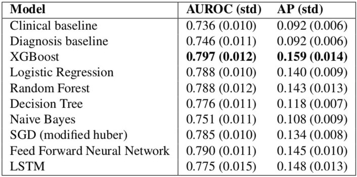
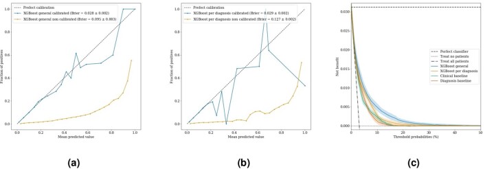
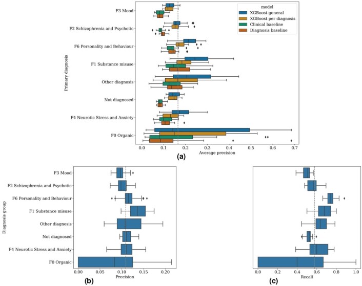
The timely identification of patients who are at risk of a mental health crisis can lead to improved outcomes and to the mitigation of burdens and costs. However, the high prevalence of mental health problems means that the manual review of complex patient records to make proactive care decisions is not feasible in practice. Therefore, we developed a machine learning model that uses electronic health records to continuously monitor patients for risk of a mental health crisis over a period of 28 days. The model achieves an area under the receiver operating characteristic curve of 0.797 and an area under the precision-recall curve of 0.159, predicting crises with a sensitivity of 58% at a specificity of 85%. A follow-up 6-month prospective study evaluated our algorithm's use in clinical practice and observed predictions to be clinically valuable in terms of either managing caseloads or mitigating the risk of crisis in 64% of cases. To our knowledge, this study is the first to continuously predict the risk of a wide range of mental health crises and to explore the added value of such predictions in clinical practice.
Overview
The claims and statistics of this paper haven’t been checked yet.
Run the check — free, no account needed. It reads the open-access text and checks the sources it cites.
Integrity signals
Registry
Cites
Statistics
Figures

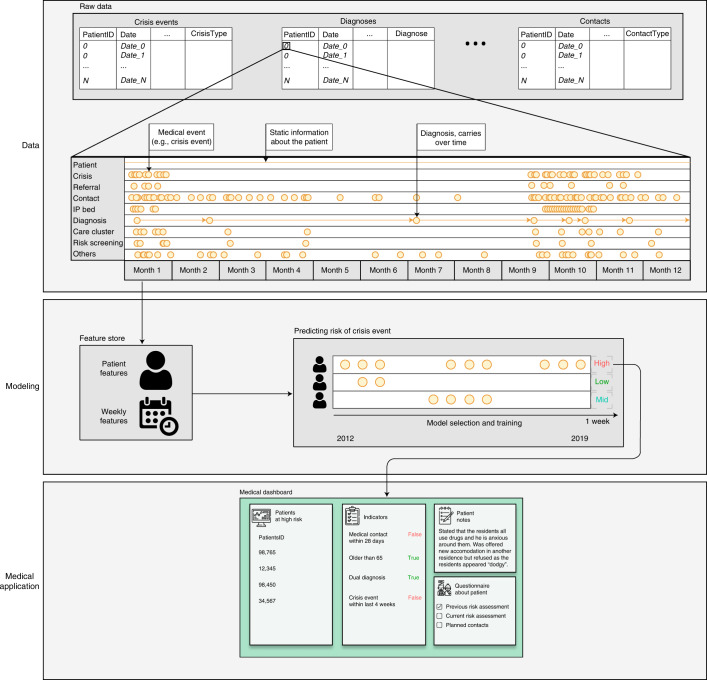
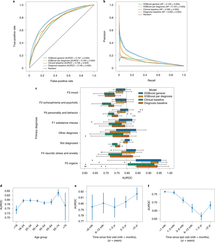
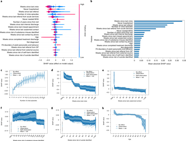
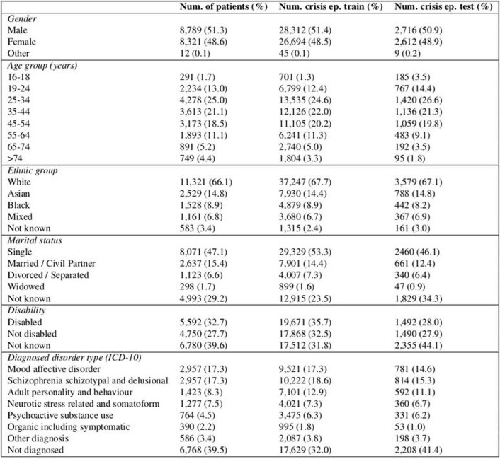
Verification
Claims the paper makes
The claims and statistics of this paper haven’t been checked yet.
Run the check — free, no account needed. It reads the open-access text and checks the sources it cites.
Claims other papers make about this one
Each is checked against this paper’s own text: does it say what the citing paper says it does?
The source backs part of the claim, not all of it — or backs it for a different population, condition or comparison.
In the citing paper
“Although predictive models show promise for improving healthcare access and quality,23 evaluative studies in applied settings are limited and primarily focus on predicting outcomes in care, not on improving provider-client fit from the start of care.24-26”
From Using Machine Learning to Match Clients and Therapy Providers: Evaluating Clinical Quality and Cost of Care (2025) · cites this paper as [26]
Experimental — accuracy not yet measured
Self-check
Percentages, sums and reported differences re-computed from the paper’s own numbers.
The self-check needs the paper’s full text.
Citations
Cites
XGBoost: A Scalable Tree Boosting System
Chen, T., & Guestrin, C. (2016) · Proceedings of the 22nd ACM SIGKDD International Conference on Knowledge Discovery and Data Mining · doi:10.1145/2939672.2939785 · Cited by 54,569
Greedy function approximation: A gradient boosting machine
Friedman, J. H. (2001) · The Annals of Statistics · doi:10.1214/aos/1013203451 · Cited by 30,731
A Unified Approach to Interpreting Model Predictions
Lundberg, S., & Lee, S.-I. (2017) · arXiv · doi:10.48550/arxiv.1705.07874 · Cited by 23,707
DeLong, E. R., DeLong, D. M., & Clarke-Pearson, D. L. (1988) · Biometrics · doi:10.2307/2531595 · Cited by 22,649
James, S. L., Abate, D., Abate, K. H., Abay, S. M., Abbafati, C., Abbasi, N., Abbastabar, H., Abd-Allah, F., Abdela, J., Abdelalim, A., et al. (2018) · The Lancet · doi:10.1016/s0140-6736(18)32279-7 · Cited by 13,867
From local explanations to global understanding with explainable AI for trees
Lundberg, S. M., Erion, G., Chen, H., DeGrave, A., Prutkin, J. M., Nair, B., Katz, R., Himmelfarb, J., Bansal, N., & Lee, S.-I. (2020) · Nature Machine Intelligence · doi:10.1038/s42256-019-0138-9 · Cited by 10,551
Decision curve analysis: a novel method for evaluating prediction models
Vickers, A. J., & Elkin, E. B. (2006) · Medical Decision Making · doi:10.1177/0272989x06295361 · Cited by 6,341
Assessing the Performance of Prediction Models: A Framework for Traditional and Novel Measures
Steyerberg, E. W., Vickers, A. J., Cook, N. R., Gerds, T., Gonen, M., Obuchowski, N., Pencina, M. J., & Kattan, M. W. (2010) · Epidemiology · doi:10.1097/ede.0b013e3181c30fb2 · Cited by 5,170
Mental health and the COVID-19 pandemic
Pfefferbaum, B., & North, C. S. (2020) · New England Journal of Medicine · doi:10.1056/nejmp2008017 · Cited by 4,378
Adaptive linear step-up procedures that control the false discovery rate
Benjamini, Y., Krieger, A. M., & Yekutieli, D. (2006) · Biometrika · doi:10.1093/biomet/93.3.491 · Cited by 3,228
Research works printed but not linked: 3
- Nielsen, D. Tree Boosting with XGBoost: Why Does XGBoost Win ‘Every’ Machine Learning Competition? Master’s thesis, Norwegian University of Science and Technology (2016).
- Bergstra, J., Yamins, D. & Cox, D. Making a science of model search: hyperparameter optimization in hundreds of dimensions for vision architectures. In: Dasgupta, S. & McAllester, D. (eds) Proc. 30th International Conference on Machine Learning, 115–123 (PMLR, 2013).
- Bergstra, J. S., Bardenet, R., Bengio, Y. & Kégl, B. Algorithms for hyper-parameter optimization. In: Shawe-Taylor, J., Zemel, R. S., Bartlett, P. L., Pereira, F. & Weinberger, K. Q. (eds) Advances in Neural Information Processing Systems 24, 2546–2554 (Curran Associates, 2011).
Cited by
Sorted by citations
Enhancing mental health with Artificial Intelligence: Current trends and future prospects
Olawade, D. B., Wada, O. Z., Odetayo, A., David-Olawade, A. C., Asaolu, F. T., & Eberhardt, J. (2024) · Journal of Medicine Surgery and Public Health · doi:10.1016/j.glmedi.2024.100099 · Cited by 667
Seiferth, C., Vogel, L., Aas, B., Brandhorst, I., Carlbring, P., Conzelmann, A., Esfandiari, N., Finkbeiner, M., Hollmann, K., Lautenbacher, H., et al. (2023) · Nature Mental Health · doi:10.1038/s44220-023-00085-1 · Cited by 105
Terra, M., Baklola, M. I., Ali, S. A. A., & El-Bastawisy, K. (2023) · The Egyptian Journal of Neurology Psychiatry and Neurosurgery · doi:10.1186/s41983-023-00681-z · Cited by 88
Islam, M. M., Hassan, S., Akter, S., Jibon, F. A., & Sahidullah, M. (2024) · Healthcare Analytics · doi:10.1016/j.health.2024.100350 · Cited by 89
Yang, Y., Song, B., Zhang, J., Dan, N., & Gu, H. (2024) · Biomacromolecules · doi:10.1021/acs.biomac.4c00803 · Cited by 69
Quantifying the impact of AI recommendations with explanations on prescription decision making
Nagendran, M., Festor, P., Komorowski, M., Gordon, A. C., & Faisal, A. A. (2023) · npj Digital Medicine · doi:10.1038/s41746-023-00955-z · Cited by 60
The use of AI in mental health services to support decision-making: scoping review
Auf, H., Svedberg, P., Nygren, J., Nair, M., & Lundgren, L. E. (2025) · Journal of Medical Internet Research · doi:10.2196/63548 · Cited by 56
Chen, J., Yuan, D., Dong, R., Cai, J., Ai, Z., & Zhou, S. (2024) · Frontiers in Psychology · doi:10.3389/fpsyg.2024.1375294 · Cited by 73
Tran, T. A., Trang, L. T. T., An, T. D., Nghĩa, N. H., & Loan, D. T. T. (2024) · Journal of Human Earth and Future · doi:10.28991/hef-2024-05-01-01 · Cited by 48
Akhlaghi, H., Freeman, S., Vari, C., McKenna, B., Braitberg, G., Karro, J., & Tahayori, B. (2024) · Emergency Medicine Australasia · doi:10.1111/1742-6723.14325 · Cited by 35
“17 developed a ML algorithm to identify patients at risk of deterioration and mental health crisis.”
MethodEstablishment of a model for predicting preterm birth based on the machine learning algorithm
Zhang, Y., Du, S., Hu, T., Xu, S., Lu, H., Xu, C., Li, J., & Zhu, X. (2023) · BMC Pregnancy and Childbirth · doi:10.1186/s12884-023-06058-7 · Cited by 44
Li, Z., Zhang, S., Huang, H., Liu, R., Cai, M., Bian, Y., Chang, L., & Du, H. (2023) · Journal of Energy Storage · doi:10.1016/j.est.2023.108926 · Cited by 39
Digital mental health care: five lessons from Act 1 and a preview of Acts 2–5
Insel, T. R. (2023) · npj Digital Medicine · doi:10.1038/s41746-023-00760-8 · Cited by 35
Schallmoser, S., Züger, T., Kraus, M., Saar‐Tsechansky, M., Stettler, C., & Feuerriegel, S. (2023) · Journal of Medical Internet Research · doi:10.2196/42181 · Cited by 35
Garriga, R., Buda, T. S., Guerreiro, J., Iglesias, J. O., Aguerri, I. E., & Matić, A. (2023) · Cell Reports Medicine · doi:10.1016/j.xcrm.2023.101260 · Cited by 36
One-Week Suicide Risk Prediction Using Real-Time Smartphone Monitoring: Prospective Cohort Study
Barrigón, M. L., Romero-Medrano, L., Moreno-Muñoz, P., Porras‐Segovia, A., López‐Castromán, J., Courtet, P., Artés-Rodrı́guez, A., & Baca‐García, E. (2023) · Journal of Medical Internet Research · doi:10.2196/43719 · Cited by 32
Requirements for Trustworthy Artificial Intelligence and its Application in Healthcare
Kim, M., Sohn, H., Choi, S. K., & Kim, S. (2023) · Healthcare Informatics Research · doi:10.4258/hir.2023.29.4.315 · Cited by 33
Ku, W. L., & Min, H. (2024) · Healthcare · doi:10.3390/healthcare12060625 · Cited by 30
War, emotions, mental health, and artificial intelligence
Ćosić, K., Kopilaš, V., & Jovanović, T. (2024) · Frontiers in Psychology · doi:10.3389/fpsyg.2024.1394045 · Cited by 58
Msosa, Y. J., Grauslys, A., Zhou, Y., Wang, T., Buchan, I. E., Langan, P., Foster, S., Walker, M., Pearson, M. G., Folarin, A., et al. (2023) · IEEE Journal of Biomedical and Health Informatics · doi:10.1109/jbhi.2023.3312011 · Cited by 29
Dhanda, S. S., Panwar, D., Lin, C., Sharma, T. K., Rastogi, D., Bindewari, S., Singh, A. M., Li, Y., Agarwal, N. K., & Agarwal, S. (2025) · Journal Of Big Data · doi:10.1186/s40537-025-01201-x · Cited by 35
Mikaeili, N., Naeim, M., & Narimani, M. (2025) · Journal of Multidisciplinary Healthcare · doi:10.2147/jmdh.s559626 · Cited by 26
Zhang, T., Tan, T., Wang, X., Gao, Y., Han, L., Balkenende, L., D'Angelo, A. R., Bao, L., Horlings, H. M., Teuwen, J., et al. (2023) · Cell Reports Medicine · doi:10.1016/j.xcrm.2023.101131 · Cited by 26
Saggu, S., Daneshvar, H., Samavi, R., Pires, P., Sassi, R. B., Doyle, T. E., Zhao, J., Mauluddin, A., & Duncan, L. (2024) · BMC Medical Informatics and Decision Making · doi:10.1186/s12911-024-02450-1 · Cited by 26
Multitask Learning for Mental Health: Depression, Anxiety, Stress (DAS) Using Wearables
Saylam, B., & İncel, Ö. D. (2024) · Diagnostics · doi:10.3390/diagnostics14050501 · Cited by 29
Ugar, E. T., & Malele, N. (2024) · Journal of Medical Ethics · doi:10.1136/jme-2023-109711 · Cited by 23
Kuang, Y., & Xie, M. (2024) · Briefings in Bioinformatics · doi:10.1093/bib/bbae464 · Cited by 22
Deep Learning based techniques for Neuro-degenerative disorders detection
Kasyap, V. L. V. S. K. B., & Dasari, C. M. (2023) · Engineering Applications of Artificial Intelligence · doi:10.1016/j.engappai.2023.106103 · Cited by 23
Biró, A., Cuesta‐Vargas, A., & Szilágyi, L. S. (2023) · Acta Universitatis Sapientiae Informatica · doi:10.2478/ausi-2023-0022 · Cited by 22
Benito, G. V., Goldberg, X., Brachowicz, N., Castaño‐Vinyals, G., Blay, N., Espinosa, A., Davidhi, F., Torres, D., Kogevinas, M., de Cid, R., et al. (2024) · Artificial Intelligence in Medicine · doi:10.1016/j.artmed.2024.102991 · Cited by 29
On the role of artificial intelligence in psychiatry
Rocheteau, E. (2022) · The British Journal of Psychiatry · doi:10.1192/bjp.2022.132 · Cited by 23
Alkhamis, M. A., Jarallah, M. A., Attur, S., & Zubaid, M. (2024) · Scientific Reports · doi:10.1038/s41598-024-51604-8 · Cited by 21
Wang, M., Sushil, M., Miao, B. Y., & Butte, A. J. (2023) · Journal of the American Medical Informatics Association · doi:10.1093/jamia/ocad085 · Cited by 21
Emotion Forecasting: A Transformer-Based Approach
Paz-Arbaizar, L., López‐Castromán, J., Artés-Rodrı́guez, A., Olmos, P. M., & Ramírez, D. (2025) · Journal of Medical Internet Research · doi:10.2196/63962 · Cited by 20
Artificial Intelligence in Mental Health Therapy for Children and Adolescents
Vial, T. M., & Almon, A. J. (2023) · Archives of Pediatrics and Adolescent Medicine · doi:10.1001/jamapediatrics.2023.4212 · Cited by 18
Assessing the impact of AI on physician decision-making for mental health treatment in primary care
Ryan, K., Yang, H., Kim, B., & Kim, J. P. (2025) · npj Mental Health Research · doi:10.1038/s44184-025-00124-y · Cited by 17
Guerreiro, J., Garriga, R., Bagén, T. L., Sharma, B., Karnik, N. S., & Matic, A. (2024) · npj Digital Medicine · doi:10.1038/s41746-024-01203-8 · Cited by 15
Mental Health Prediction using Machine Learning Models and Large Language Model
Kamoji, S., Rozario, S., Almeida, S., Patil, S., Patankar, S. S., & Pendhari, H. (2024) · International Conference on Inventive Computing and Informatics (ICICI) · doi:10.1109/icici62254.2024.00040 · Cited by 14
Predicting depression in old age: Combining life course data with machine learning
Montorsi, C., Fusco, A., Kerm, P. V., & Bordas, S. (2023) · Economics & Human Biology · doi:10.1016/j.ehb.2023.101331 · Cited by 15
Feng, W., Wu, H., Ma, H., Tao, Z., Xu, M., Zhang, X., Lü, S., Wan, C., & Liu, Y. (2023) · Journal of the American Medical Informatics Association · doi:10.1093/jamia/ocad228 · Cited by 13
Qi, C., Hu, T., Zheng, J., Li, K., Zhou, M., Zhou, M., & Chen, Q. (2024) · Environmental Research · doi:10.1016/j.envres.2024.118378 · Cited by 13
Ajayi, S. O., Dolla, T. H., Sikeyi, L. L., Akinola, A. O., Maboya, W. K., Liu, X., Makgwane, P. R., & Mathe, M. K. (2024) · Materials Today Sustainability · doi:10.1016/j.mtsust.2024.100899 · Cited by 14
Automated machine learning for classification and regression: A tutorial for psychologists
Lee, C., & Gates, K. M. (2025) · Behavior Research Methods · doi:10.3758/s13428-025-02684-5 · Cited by 12
Osorio, J., Figueroa, M., & Wong, L. (2024) · Journal of Computer Science · doi:10.3844/jcssp.2024.181.190 · Cited by 12
Machine Learning for Mental Health: Applications, Challenges, and the Clinician's Role
Singhal, S., Cooke, D. L., Villareal, R. I., Stoddard, J., Lin, C., & Dempsey, A. G. (2024) · Current Psychiatry Reports · doi:10.1007/s11920-024-01561-w · Cited by 13
Jiang, Z., Cui, Y., Xu, H., Abbey, C., Xu, W., Guo, W., Zhang, D., Liu, J., Jin, J., & Li, Y. (2024) · Annals of General Psychiatry · doi:10.1186/s12991-024-00534-w · Cited by 14
Wang, P., Liu, H., Shi, Y., Liu, A., Zhu, Q., Albu, I., Pacholec, M., Cheng, L. L., Sun, X. S., & Chi, X. (2025) · Med Research · doi:10.1002/mdr2.70017 · Cited by 18
Wenzl, F. A., Ow, K. W., Velders, M. A., Tyrer, F., Paley, L., Lai, J. H., Smolle, M. A., Schweiger, V., Hagström, E., de Belder, M., et al. (2026) · The Lancet · doi:10.1016/s0140-6736(25)02020-3 · Cited by 12
Real Time Mental Health Monitoring System using Machine Learning
Venkataramanaiah, B., Reddy, K. G., Satheesh Kumar, S., RAMAKRISHNAN, K., M, S., & Rajesh, S. (2024) · International Conference on Intelligent Cyber Physical Systems and Internet of Things (ICoICI) · doi:10.1109/icoici62503.2024.10696460 · Cited by 11
Liu, X., Shu, X., Zhou, Y., & Jiang, Y. (2024) · Frontiers in Oncology · doi:10.3389/fonc.2024.1499794 · Cited by 11
Kim, S., Kim, H., Kim, S., Lee, H., Hammoodi, A., Choi, Y., Kim, H. J., Smith, L., Kim, M. S., Fond, G. B., et al. (2025) · Journal of Medical Internet Research · doi:10.2196/62805 · Cited by 11
Șerban, M., Toader, C., & Covache-Busuioc, R.-A. (2025) · International Journal of Molecular Sciences · doi:10.3390/ijms26178114 · Cited by 16
Otsuka, N., Kawanishi, Y., Doi, F., Takeda, T., Okumura, K., Yamauchi, T., Yada, S., Wakamiya, S., Aramaki, E., & Makinodan, M. (2023) · Psychiatry and Clinical Neurosciences · doi:10.1111/pcn.13580 · Cited by 10
Lee, J. L., Billovits, C., Chen, S.-Y., Wickham, R. E., Kocher, B., Chen, C. E., & Lungu, A. (2025) · Value in Health · doi:10.1016/j.jval.2025.06.002 · Cited by 8
Wang, G., Bennamoun, H., Kwok, W. H., Quimbayo, J. P. O., Kelly, B., Ratajczak, T., Marriott, R., Walker, R., & Kotz, J. (2025) · Journal of Medical Internet Research · doi:10.2196/68030 · Cited by 10
Prediction of Psychiatric Disorders Using Deep Learning
Gurrapu, O., Reddy, C. K., Saripalli, A. K., Mannanuddin, K., Swamy, G. V., Naick, B. R., Venkataramanaiah, B., & Suman, J. V. (2025) · International Conference on Inventive Systems and Control (ICISC) · doi:10.1109/icisc65841.2025.11187494 · Cited by 8
Tay, J. L., Htun, K. K., & Sim, K. (2024) · Brain Sciences · doi:10.3390/brainsci14090878 · Cited by 7
Application of Predictive Analytics in Pregnancy, Birth, and Postpartum Nursing Care
Dreisbach, C., Barcelona, V., Turchioe, M. R., Bernstein, S., & Erickson, E. N. (2024) · MCN The American Journal of Maternal/Child Nursing · doi:10.1097/nmc.0000000000001082 · Cited by 8
Jin, J. J., Yu, L., Zhou, Q., Du, Q., Nie, X., Yin, H., & Gu, W. (2025) · Frontiers in Cellular and Infection Microbiology · doi:10.3389/fcimb.2025.1569748 · Cited by 7
Al-Juhani, A. A., Desoky, R. M., Iskander, Z., Alotaibi, R. M., Alzain, N. N., AlJohani, N. I., Alrefaai, M. M., Alhasanat, R. A., AlMehaimeed, M. A., & Alharthi, A. S. (2025) · Cureus · doi:10.7759/cureus.89873 · Cited by 7
Investigations on Machine Learning Models for Mental Health Analysis and Prediction
Ajith Sankar, R., & Juliet, S. (2023) · International Conference on Electrical, Electronics, Information and Communication Technologies (ICEEICT) · doi:10.1109/iceeict56924.2023.10157385 · Cited by 7
Zhang, Y. (2024) · American Journal of Cancer Research · doi:10.62347/lndl8700 · Cited by 7
Hua, Y., Blackley, S. V., Shinn, A. K., Skinner, J. P., Moran, L. V., & Zhou, L. (2025) · Translational Psychiatry · doi:10.1038/s41398-025-03629-4 · Cited by 5
A Machine Learning Approach to Mental Disorder Prediction: Handling the Missing Data Challenge
Mokheleli, T., Bokaba, T., Museba, T., & Ntshingila, N. (2024) · Lecture notes of the Institute for Computer Sciences, Social Informatics and Telecommunications Engineering · doi:10.1007/978-3-031-63999-9_6 · Cited by 6
Zhu, S., Tan, X., Huang, H., Zhou, Y., & Liu, Y. (2024) · Heliyon · doi:10.1016/j.heliyon.2024.e35586 · Cited by 6
Flexible imputation toolkit for electronic health records
Sadr, A. V., Li, J., Hwang, W., Yeasin, M., Wang, M., Lehmann, H. P., Zand, R., & Abedi, V. (2025) · Scientific Reports · doi:10.1038/s41598-025-02276-5 · Cited by 9
AI Integration in Behavioral Healthcare: A Practical Framework for Clinicians
Sadeh‐Sharvit, S., & Hollon, S. D. (2025) · Journal of Technology in Behavioral Science · doi:10.1007/s41347-025-00532-z · Cited by 8
The Use of Artificial Intelligence for Personalized Treatment in Psychiatry
Jalali, S., You, Q., Xu, V., Chen, L., Zini, J., Zamorano, T., Luo, Y., Friesen, T., Fontana, G. J., & Benrimoh, D. A. (2025) · Current Psychiatry Reports · doi:10.1007/s11920-025-01656-y · Cited by 8
The potential of depressive symptoms to identify cognitive impairment in ageing
Alexopoulos, P., Bountoulis, C., Katirtzoglou, E. A., Kosmidis, M. H., Siarkos, K., Yannakoulia, M., Dardiotis, E., Skondra, M., Hadjigeorgiou, G. M., Perneczky, R., et al. (2025) · European Journal of Ageing · doi:10.1007/s10433-025-00837-1 · Cited by 6
Hudon, A., Beaudoin, M., Phraxayavong, K., Potvin, S., & Dumais, A. (2023) · Journal of Personalized Medicine · doi:10.3390/jpm13121660 · Cited by 7
Omae, Y., Sakai, Y., & Takahashi, H. (2023) · AIMS Mathematics · doi:10.3934/math.2024041 · Cited by 5
Longitudinal analysis of adolescents at high risk of depression: Prediction models
Park, J., Choi, E. K., & Choi, M. (2025) · Applied Nursing Research · doi:10.1016/j.apnr.2025.151927 · Cited by 5
Yan, Y. (2024) · International Journal of Human-Computer Interaction · doi:10.1080/10447318.2024.2320981 · Cited by 5
RetractedOptimization of potential targets for antidepressant Chinese medicines: AI and multi-omics methods
Lei, C., Chen, Z., Ma, C., Xie, L., Wu, D., Chen, J., & Chen, J. (2026) · Chinese Medicine · doi:10.1186/s13020-025-01320-w · Cited by 5
Wang, H., Yang, C., Zhao, M., Ren, F.-G., Wang, X., Yan, H., QIN, W., Tian, F., & Li, L. (2026) · Microbiology Spectrum · doi:10.1128/spectrum.03713-25 · Cited by 3
Abudurexiti, N., Liu, B., Wang, S., Dong, Q., Batuer, M., Liu, Z., & Li, X. (2025) · Journal of Inflammation Research · doi:10.2147/jir.s518631 · Cited by 4
Park, Y. H., Kim, Y. W., Kang, D. R., Lee, S. C., & Yoon, S. Y. (2025) · npj Parkinson s Disease · doi:10.1038/s41531-025-01007-x · Cited by 4
Nazih, W., Abuhmed, T., Alharbi, M., & El–Sappagh, S. (2025) · PLoS ONE · doi:10.1371/journal.pone.0332134 · Cited by 5
Predicting Mental Health Crises Using Social Media Sentiment Analysis: A Machine Learning Approach
Narang, G., & Marken, G. (2025) · International Conference on Computing Technologies & Data Communication (ICCTDC) · doi:10.1109/icctdc64446.2025.11158851 · Cited by 4
Moudden, I. E., Bittner, M. L., Karpov, M. V., Osunmakinde, I. O., Acheamponmaa, A., Jackson-Nevels, B., Mbaye, M. T., Fields, T. L., Jordan, K., & Bahoura, M. J. (2025) · Scientific Reports · doi:10.1038/s41598-025-89579-9 · Cited by 5
Zugman, A., Ringlein, G., Finn, E. S., Lewis, K. M., Berman, E., Silverman, W. K., Lebowitz, E. R., Pine, D. S., & Winkler, A. M. (2025) · Psychological Medicine · doi:10.1017/s0033291724003131 · Cited by 3
Rajaram, G., Vedavalli, S., Sivakumar, V. G., Varshini, D. R. S., J, C. M. B. M., & Shaby, S. M. (2025) · International Conference on Trends in Electronics and Informatics (ICOEI) · doi:10.1109/icoei65986.2025.11013632 · Cited by 3
Zhao, S., Li, X., Gao, X., Lv, Y., Cao, Y., Mi, G., Wang, H., Niu, L., & Li, Y. (2025) · Child and Adolescent Psychiatry and Mental Health · doi:10.1186/s13034-025-00969-3 · Cited by 3
Fernández-Quijano, I., Herrera‐Peco, I., López‐Espuela, F., Suárez-Llevat, C., Moreno-Sánchez, R., & Ruíz-Núñez, C. (2025) · Psychiatry International · doi:10.3390/psychiatryint6040143 · Cited by 3
Pal, S., & Karmakar, R. (2026) · Lecture notes in computer science · doi:10.1007/978-3-032-15621-1_19 · Cited by 3
Lancashire, L., Lancaster, S. L., Linkh, D. J., Hassan, A. M., Haas, M., & Gage, A. T. (2024) · Journal of Psychiatric Research · doi:10.1016/j.jpsychires.2024.12.007 · Cited by 4
Liu, L., Jiang, J., Wu, L., Zeng, D. M., Yan, C., Liang, L., Shi, J., & Xie, Q. (2024) · PeerJ · doi:10.7717/peerj.17164 · Cited by 3
Rashid, S., Badrul, T., Rafid, L., Setu, J. H., Halder, N., & Islam, A. (2024) · Advances in Science and Engineering Technology International Conferences (ASET) · doi:10.1109/aset60340.2024.10708680 · Cited by 3
GRU-TV: Time- and Velocity-aware Gated Recurrent Unit for patient representation
Liu, N., Gou, S., Gao, R., Su, B., Liu, W., Park, C., Xing, S., Yuan, J. Y., & Fenster, A. (2025) · Journal of Biomedical Informatics · doi:10.1016/j.jbi.2025.104855 · Cited by 2
Taquet, M., Fazel, S., & Rush, A. J. (2025) · BMJ Mental Health · doi:10.1136/bmjment-2025-301622 · Cited by 2
Apply Machine Learning to Predict Risk for Adolescent Depression in a Cohort of Kenyan Adolescents
Do, H., Huang, K., Cheng, S., Njiru, L. N., Mwavua, S., Obondo, A., & Kumar, M. (2025) · Healthcare · doi:10.3390/healthcare13202620 · Cited by 4
Hou, X., Deng, Z., Zhou, Y., Hong, J., Wu, F., Li, Y., Huang, J., Dai, C., Lu, L., Tang, G., et al. (2025) · MedComm · doi:10.1002/mco2.70444 · Cited by 2
Rao, K. S., Rajasekaran, V., Kotoju, R., & Shankar, L. S. (2025) · Lecture notes in networks and systems · doi:10.1007/978-981-96-9242-2_41 · Cited by 2
Hummel, L., Lorenz-Artz, K. C. A. G., Bierbooms, J. J. P. A., & Bongers, I. M. B. (2025) · JMIR Medical Informatics · doi:10.2196/74240 · Cited by 4
He, H., Ying, Z., Li, B., Fan, Y., Wang, P., Lu, J., Wu, L., Zhao, H., Guo, Y., Wang, G., et al. (2026) · Communications Medicine · doi:10.1038/s43856-026-01449-1 · Cited by 2
Liang, L., Lu, X., Jiao, D., Xiao, B., Fang, S. H. A. N., Zhang, R., Zhao, C., & Song, J. (2026) · BMC Psychiatry · doi:10.1186/s12888-026-08190-y · Cited by 2
Machine Learning based Self Identification of Mental Health
Poornima, S., Agalya, R., Gayathri, M., Hari, A., & Sudharsan, S. (2024) · International Conference on IoT, Communication and Automation Technology (ICICAT) · doi:10.1109/icicat62666.2024.10923396 · Cited by 2
A Self-Stabilizing and Parameter-Optimized Deep Learning Model for Predicting Mental Health Disorder
(2022) · International journal of intelligent engineering and systems · doi:10.22266/ijies2022.1231.49 · Cited by 2
Cosic, K., Kuljanac, A., & Palermo, S. (2026) · Frontiers in psychology · doi:10.3389/fpsyg.2026.1821242 · Cited by 3
“…enhance the prediction of human mental readiness and performance by analyzing complex patterns of large neuro-psycho-physiological datasets, operational context and human performance during startle operations (Chen et al., 2022; Garriga et al., 2022; Le Glaz et al., 2021; Sabry et al., 2022).”
Metadata
- Authors
- Garriga, R., Mas, J., Abraha, S., Nolan, J., Harrison, O., Tadros, G., & Matic, A.
- Affiliations
- Universitat Pompeu Fabra (ES)
- Birmingham and Solihull Mental Health NHS Foundation Trust (GB)
- Aston University (GB)
- Corresponding author
- Garriga, Roger
- Matic, Aleksandar
- Venue
- Nature Medicine
- Published
- 2022-05-16
- Volume
- 28
- Issue
- 6
- Pages
- 1240-1248
- ISSN
- 1078-8956 (ISSN-L)
- 1546-170X
- PMC
- PMC9205775
- OpenAlex
- W4280536523
- Cited by
- 229
- References
- 56
- Citations by year
- 2026: 56 · 2025: 90 · 2024: 46 · 2023: 33 · 2022: 4
- FWCI
- 14.18
- Type
- journal article
- Language
- en
- Open access
- hybrid
- doi.org
- Locations
- Nature Medicine (publishedVersion, cc-by)
- Research Square (acceptedVersion, cc-by)
- PubMed Central (publishedVersion, cc-by)
- PubMed (publishedVersion)
- Aston Publications Explorer (Aston University) (acceptedVersion)
- Warwick Research Archive Portal (University of Warwick) (acceptedVersion)
- Funders
- Health Foundation (709246)
- Topics
- Physical Sciences › Computer Science › Artificial Intelligence › Machine Learning in Healthcare
- Social Sciences › Psychology › Social Psychology › Mental Health via Writing
- Health Sciences › Health Professions › Health Information Management › Artificial Intelligence in Healthcare
- Keywords
- electronic health records, risk prediction, clinical decision support, continuous patient monitoring, clinical utility, mental health services
- MeSH terms
- Machine Learning, Humans, Mental Health, Prospective Studies, ROC Curve, Electronic Health Records
About these checks
Registry, retraction, Cites and statistics results are computed, not judged, with one exception: a printed reference that no index lists is read once by a model before it counts as a citation error. Claims are extracted by a model and kept only when their quote appears verbatim in the text; each cited source is then checked, with a model’s help, for whether it says what the claim relies on. Those verdicts can be wrong — read the claim’s quote and the cited source before relying on one.
Statistics and arithmetic are recomputed, not judged.
Confidence bands are shown only for fields calibrated on our annotated test set. None is calibrated yet, so no band is shown.
What counts as a claim ›How we measure confidence ›How we check this ›
Are you an author, or do you see a problem with this page? Request a review
