

The DOI matches its Crossref record; 64 of the 66 references it cites were found in a registry or an index.
Machine learning for comprehensive forecasting of Alzheimer’s Disease progression
Open accessAbstract
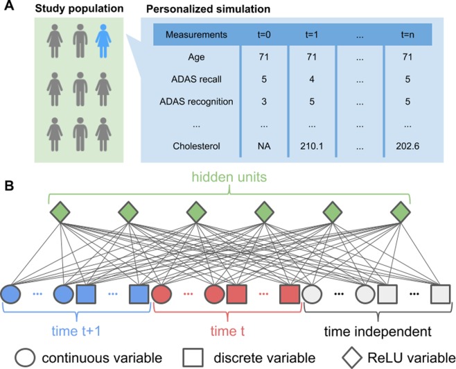
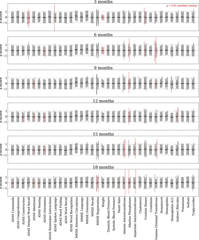
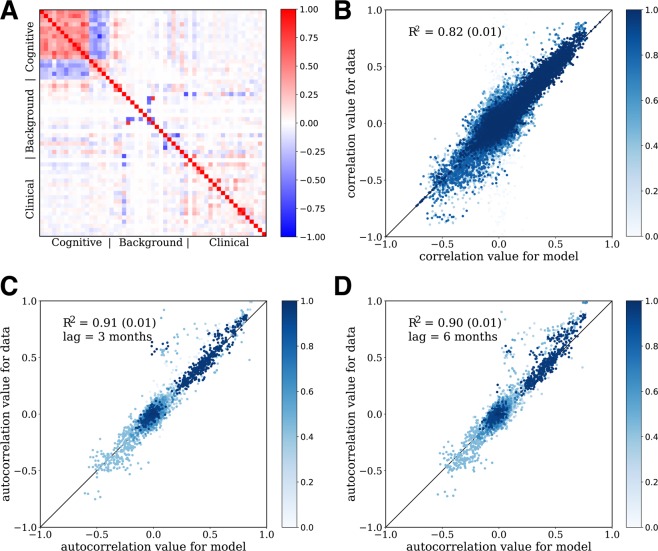
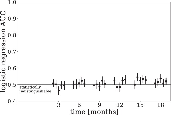
Most approaches to machine learning from electronic health data can only predict a single endpoint. The ability to simultaneously simulate dozens of patient characteristics is a crucial step towards personalized medicine for Alzheimer’s Disease. Here, we use an unsupervised machine learning model called a Conditional Restricted Boltzmann Machine (CRBM) to simulate detailed patient trajectories. We use data comprising 18-month trajectories of 44 clinical variables from 1909 patients with Mild Cognitive Impairment or Alzheimer’s Disease to train a model for personalized forecasting of disease progression. We simulate synthetic patient data including the evolution of each sub-component of cognitive exams, laboratory tests, and their associations with baseline clinical characteristics. Synthetic patient data generated by the CRBM accurately reflect the means, standard deviations, and correlations of each variable over time to the extent that synthetic data cannot be distinguished from actual data by a logistic regression. Moreover, our unsupervised model predicts changes in total ADAS-Cog scores with the same accuracy as specifically trained supervised models, additionally capturing the correlation structure in the components of ADAS-Cog, and identifies sub-components associated with word recall as predictive of progression.
Overview
The claims and statistics of this paper haven’t been checked yet.
Run the check — free, no account needed. It reads the open-access text and checks the sources it cites.
Integrity signals
Registry
Cites
Statistics
Figures
Verification
Claims the paper makes
The claims and statistics of this paper haven’t been checked yet.
Run the check — free, no account needed. It reads the open-access text and checks the sources it cites.
Claims other papers make about this one
Each is checked against this paper’s own text: does it say what the citing paper says it does?
The source backs part of the claim, not all of it — or backs it for a different population, condition or comparison.
In the citing paper
“From a commercial point of view, Unlearn.AI has developed and tested digital twin models that leverage diverse sets of clinical data to enhance clinical trials for Alzheimer's disease and multiple sclerosis 70,71 .”
From Multimodal biomedical AI (2022) · cites this paper as [70]
Experimental — accuracy not yet measured
Self-check
Percentages, sums and reported differences re-computed from the paper’s own numbers.
The self-check needs the paper’s full text.
Citations
Cites
Statistical Power Analysis for the Behavioral Sciences
Muller, K. E., & Cohen, J. (1989) · Technometrics · doi:10.2307/1270020 · Cited by 99,603
Folstein, M. F., Folstein, S. E., & McHugh, P. R. (1975) · Journal of Psychiatric Research · doi:10.1016/0022-3956(75)90026-6 · Cited by 88,282
Statistical power analysis for the behavioral sciences
Cohen, J. (1990) · Computers Environment and Urban Systems · doi:10.1016/0198-9715(90)90050-4 · Cited by 65,417
Hirono, N., Mori, E., Ikejiri, Y., Imamura, T., Shimomura, T., Hashimoto, M., Yamashita, H., & Ikeda, M. (1997) · PubMed · Cited by 21,012
Kok, J. S., Berg, I. J., & Scherder, E. J. A. (2013) · Dementia and Geriatric Cognitive Disorders Extra · doi:10.1159/000353441 · Cited by 20,589
Older Adults' Reasons for Using Technology while Aging in Place
Peek, S. T. M., Luijkx, K. G., Rijnaard, M. D., Nieboer, M. E., van der Voort, C. S., Aarts, S., van Hoof, J., Vrijhoef, H. J., & Wouters, E. (2015) · Gerontology · doi:10.1159/000430949 · Cited by 19,852
Sensitivity and False Alarm Rate of a Fall Sensor in Long-Term Fall Detection in the Elderly
Kangas, M., Korpelainen, R., Vikman, I., Nyberg, L., & Jämsä, T. J. (2014) · Gerontology · doi:10.1159/000362720 · Cited by 19,007
Advances in Neural Information Processing Systems 19
(2007) · The MIT Press eBooks · doi:10.52202/085713 · Cited by 16,043
Proceedings of the 24th international conference on Machine learning
(2007) · doi:10.1145/1273496 · Cited by 11,869
A New Initiative on Precision Medicine
Collins, F. S., & Varmus, H. (2015) · New England Journal of Medicine · doi:10.1056/nejmp1500523 · Cited by 5,202
Research works printed but not linked: 2
- th International Symposium on, 1015-1018 (IEEE, 2014).
- Dankar, F. K. & El Emam, K. Practicing differential privacy in health care: A review. Transactions on Data Priv. 6, 35–67 (2013).
Cited by
Sorted by citations
Items 201–222 of 222
Farhat, H., Abid, C., Alinier, G., Khadhraoui, M., Gargouri, I., Shaikh, L. A. H. A., & Laughton, J. (2025) · BMC Emergency Medicine · doi:10.1186/s12873-025-01340-7
Development of digital twin models for heart failure patient treatment
Lei, H., & Chang, A. C. (2025) · Elsevier eBooks · doi:10.1016/b978-0-443-13279-7.00052-3
AI in Diagnostics and Treatment Planning
Panigrahy, U. P., Verma, A., SHARMA, A. K., Sharma, S., & Sagapola, R. (2025) · BENTHAM SCIENCE PUBLISHERS eBooks · doi:10.2174/9798898811563125010009
Foundations of AI in Modern Neuroscience
Rudroff, T. (2025) · Neurocultural health and wellbeing · doi:10.1007/978-3-032-11596-6_1
Chen, R., Bartelo, N., Arikatla, M. R., Mason, C. E., & Elemento, O. (2025) · medRxiv · doi:10.1101/2025.11.27.25341167
Batlle, P., Darcy, M. D., Levine, M., Hamzi, B., Owhadi, H., Bastani, M., Zhang, Y., Sarsour, K., Talamas, F., & Database, F. T. C. (2025) · Journal of Alzheimer s Disease · doi:10.1177/13872877251404082
Kim, J., Lee, H., Lee, J., Rhee, S. Y., Shin, J. I., Lee, S. W., Cho, W., Min, C., Kwon, R., Kim, J. G., et al. (2023) · Figshare · doi:10.6084/m9.figshare.23733093
The Change in Dementia Presentation During the Past Decades
Jhang, K.-M., Lee, C.-J., & Chen, Y.-C. (2026) · Springer eBooks · doi:10.1007/978-981-95-5222-1_11
PINN-EM: Physics-Guided Disease Progression Model of Geographic Atrophy
Lachinov, D., Pinetz, T., & Bogunović, H. (2026) · IEEE Transactions on Biomedical Engineering · doi:10.1109/tbme.2026.3655164
Introduction of Artificial Intelligence in Healthcare
Tayebi, L., Shetty, S. P., & Imani, S. (2026) · Springer eBooks · doi:10.1007/978-3-032-15977-9_1 · Cited by 1
Xiong, X., Wang, X., Zhu, C., He, J., & Initiative, A. D. N. (2026) · PLoS ONE · doi:10.1371/journal.pone.0342549
Singh, S., Sharma, Y., Bhardwaj, P., Kothari, D., Chhikara, A., Gupta, V., Kumar, D., Choudhary, N., & Kondaveeti, S. B. (2026) · Behavioral and Brain Functions · doi:10.1186/s12993-026-00329-x · Cited by 2
RBXRT++: A New Data-Driven Approach for Detecting Alzheimer's and Cognitive Decline
Manik, M. M. T. G., Rahman, R., Tasnim, A. F., Nilima, S. I., Yeasmin, S., Das, S., & Akhter, F. (2025) · International Conference on Electrical, Computer and Energy Technologies (ICECET) · doi:10.1109/icecet63943.2025.11472184
Kiakou, D., Mueller, K., Filip, P., Lasica, A., Hofmann, S., Růžička, F., Urgošík, D., Burdová, K., & Jech, R. (2026) · IEEE Transactions on Neural Systems and Rehabilitation Engineering · doi:10.1109/tnsre.2026.3682582
Transition-Based Digital Twin Modelling for Alzheimer’s Disease Under Sparse Longitudinal Data
Huang, Y., Zhang, Y., Michopoulou, S. K., Kipps, C., & Attar, R. (2026) · Lecture notes in computer science · doi:10.1007/978-3-032-35390-0_15
Castagno, S., Subramanian, A., Epanomeritakis, I. E., Gompels, B., McDonnell, S., Birch, M., van der Schaar, M., & McCaskie, A. W. (2026) · Journal of the American Medical Informatics Association · doi:10.1093/jamia/ocag102
Data Stewardship Barriers to Building Digital Twin Technology for Precision Medicine
Silva, P. J., Tao, J., Rogers, S. L., He, Q., Robert, J. D., Black, L., Bruce, S. A., Shireman, P. K., & Ramos, K. S. (2026) · AI in Medicine · doi:10.3390/aimed1030020
Deep learning in neurological disease and brain health: foundations, applications, and challenges
Mohan, N. J., Murugan, R., & Goel, T. (2026) · Elsevier eBooks · doi:10.1016/b978-0-44-330291-6.00010-x
AI Cautionary Guide: Pitfalls and Strategies for the Use of Machine Learning in Medical Research
Liu, Q., Huang, R., Zhang, H., & Osborne, T. F. (2026) · Clinical Pharmacology & Therapeutics · doi:10.1002/cpt.70469
Fawaz, A. (2026) · Research Square · doi:10.21203/rs.3.rs-10940313/v1
Omidi, M., Bacsu, J.-D., Absher, J. R., Babaieasl, F., Kooshiar, H., Imani, S. M., Ebrahimi, N., Smith, M. L., & Rahemi, Z. (2026) · Bioengineering · doi:10.3390/bioengineering13101225
ÇİÇİN, F. N. (2026) · Therapeutic Innovation & Regulatory Science · doi:10.1007/s43441-026-01067-y
Metadata
- Authors
- Fisher, C. K., Smith, A. M., Walsh, J. R., Diseases, C. A. M., Simon, A. J., Edgar, C., Jack, C. R., Holtzman, D., Russell, D., Hill, D., Grosset, D., Wood, F., Vanderstichele, H., Morris, J., Blennow, K., Marek, K., Shaw, L. M., Albert, M., Weiner, M., Fox, N., Aisen, P., Cole, P. E., Petersen, R., Sherer, T., Kubick, W., & Abbott, A. F. A. R.
- Affiliations
- Mayo Clinic (US)
- Washington University in St. Louis (US)
- Institute for Neurodegenerative Disorders (US)
- University of Glasgow (GB)
- Fujirebio (Belgium) (BE)
- Johns Hopkins University (US)
- University of California, San Francisco (US)
- University College London (GB)
- Michael J. Fox Foundation (US)
- Corresponding author
- Fisher, Charles K.
- ORCID
- Venue
- Scientific Reports
- Published
- 2019-09-20
- Volume
- 9
- Issue
- 1
- Pages
- 13622-13622
- ISSN
- 2045-2322 (ISSN-L)
- PMC
- PMC6754403
- OpenAlex
- W2974138729
- Cited by
- 223
- References
- 66
- Citations by year
- 2026: 22 · 2025: 37 · 2024: 30 · 2023: 39 · 2022: 33 · 2021: 27 · 2020: 32 · 2019: 3
- FWCI
- 18.92
- Type
- journal article
- Language
- en
- Open access
- gold
- doi.org
- Locations
- Scientific Reports (publishedVersion, cc-by)
- PubMed Central (publishedVersion, cc-by)
- PubMed (publishedVersion)
- arXiv (Cornell University) (submittedVersion)
- DOAJ (DOAJ: Directory of Open Access Journals) (submittedVersion)
- UCL Discovery (University College London) (submittedVersion)
- eScholarship (California Digital Library) (submittedVersion, cc-by)
- arXiv (Cornell University)
- Topics
- Health Sciences › Medicine › Psychiatry and Mental health › Dementia and Cognitive Impairment Research
- Physical Sciences › Computer Science › Artificial Intelligence › Machine Learning in Healthcare
- Health Sciences › Health Professions › Health Information Management › Artificial Intelligence in Healthcare
- Keywords
- Alzheimer's disease progression, mild cognitive impairment, conditional restricted Boltzmann machine, ADAS-Cog, word recall, cognitive decline prediction
- MeSH terms
- Machine Learning, Aged, Aged, 80 and over, Alzheimer Disease, Cognition, Female, Forecasting, Humans, Male, Middle Aged, Models, Theoretical, Neuropsychological Tests, Models, Statistical, Disease Progression, Cognitive Dysfunction
About these checks
Registry, retraction, Cites and statistics results are computed, not judged, with one exception: a printed reference that no index lists is read once by a model before it counts as a citation error. Claims are extracted by a model and kept only when their quote appears verbatim in the text; each cited source is then checked, with a model’s help, for whether it says what the claim relies on. Those verdicts can be wrong — read the claim’s quote and the cited source before relying on one.
Statistics and arithmetic are recomputed, not judged.
Confidence bands are shown only for fields calibrated on our annotated test set. None is calibrated yet, so no band is shown.
What counts as a claim ›How we measure confidence ›How we check this ›
Are you an author, or do you see a problem with this page? Request a review
