

The DOI matches its Crossref record.
Magnetic hopfions in solids
Abstract
Hopfions are an intriguing class of string-like solitons, named according to a classical topological concept classifying three-dimensional direction fields. The search for hopfions in real physical systems has been ongoing for nearly half a century, starting with the seminal work of Faddeev. However, so far, realizations in bulk solids are missing. Here, we show that hopfions appear as emergent particles of the classical Heisenberg model with competing exchange interactions. This requires going beyond the model approach used in prior work and deriving a general micromagnetic energy functional directly from a spin-lattice Hamiltonian. We present a definite parameter space in which the existence of hopfions is possible. This opens a concrete vista to combine computational approaches such as density functional theory with material informatics to find magnetic crystals that can host hopfions. As proof of principle, we show how zero-field hopfions can be visualized by the means of off-axis electron holography in a transmission electron microscope.
Overview
The claims and statistics of this paper haven’t been checked yet.
Run the check — free, no account needed. It reads the open-access text and checks the sources it cites.
Integrity signals
Registry
Cites
Statistics
Figures
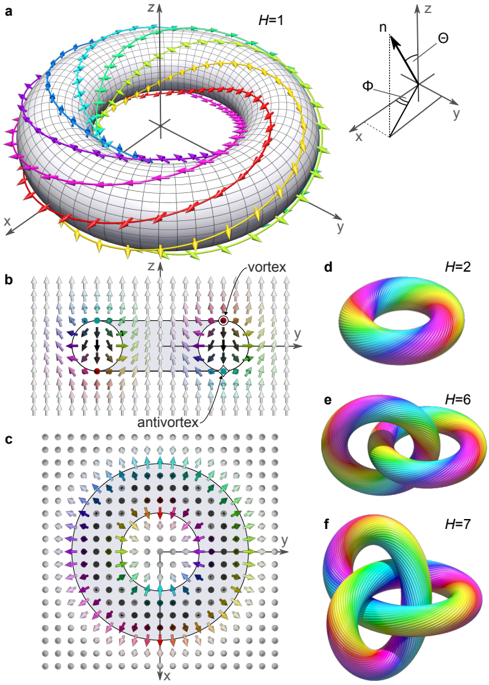
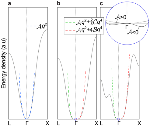
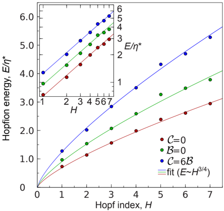
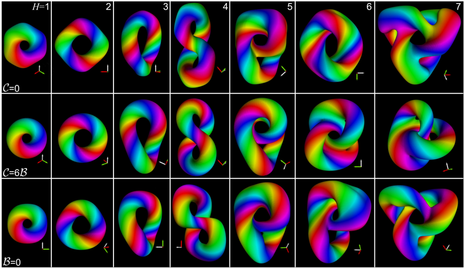
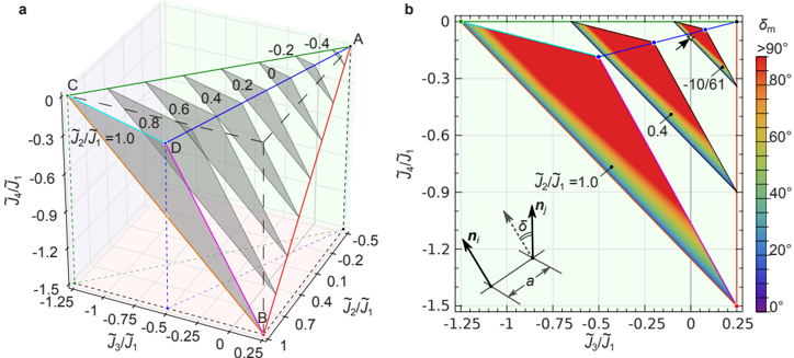
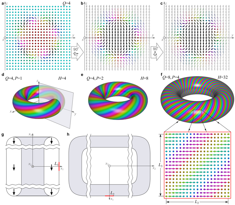
Verification
Claims the paper makes
The claims and statistics of this paper haven’t been checked yet.
Run the check — free, no account needed. It reads the open-access text and checks the sources it cites.
Claims other papers make about this one
Each is checked against this paper’s own text: does it say what the citing paper says it does?
The check wasn’t confident either way, so it gives no verdict — never disputed.
In the citing paper
“In parallel, a stable, individual skyrmions formed by the spin distribution of a SPP field in the presence of spin-orbit coupling was demonstrated [19].”
From Optical skyrmions and other topological quasiparticles of light (2024) · cites this paper as [19]
Experimental — accuracy not yet measuredThe check wasn’t confident either way, so it gives no verdict — never disputed.
In the citing paper
“Optical plasmonic field-and spin-skyrmions were verified to possess deep-subwavelength features with sufficient light intensities [19,40], which meets the emerging requirements of superresolution imaging and metrology.”
From Optical skyrmions and other topological quasiparticles of light (2024) · cites this paper as [19]
Experimental — accuracy not yet measuredThe check wasn’t confident either way, so it gives no verdict — never disputed.
In the citing paper
“(i) ultrasmall-the spatial size of a spin-skyrmion features can be realized on a deep-subwavelength scale as the spin is not subject to diffraction [19,40,51]”
From Optical skyrmions and other topological quasiparticles of light (2024) · cites this paper as [19]
Experimental — accuracy not yet measuredIn the citing paper
“Very recently, skyrmionic structures were observed in optics [18,19].”
From Optical skyrmions and other topological quasiparticles of light (2024) · cites this paper as [19]
In the citing paper
“Such optical skyrmions are most closely related to their magnetic counterparts and can exist as individual isolated quasiparticles [19] as well as form hexagonal lattices [46].”
From Optical skyrmions and other topological quasiparticles of light (2024) · cites this paper as [19]
In the citing paper
“The same as the field-skyrmions, optical spin-skyrmions also allow only Néel-type textures in the isotropic medium (Fig. 4b) [19].”
From Optical skyrmions and other topological quasiparticles of light (2024) · cites this paper as [19]
In the citing paper
“The spin vectors in a tightly focused vortex beam may look like a Néel-type skyrmion-like texture in the focal plane near the beam axis, however, it is not a rigorous analogue of a skyrmion and a skyrmion number can not be assigned [19].”
From Optical skyrmions and other topological quasiparticles of light (2024) · cites this paper as [19]
In the citing paper
“The radial kπ-twist structures of the spin-skyrmion possess deep-subwavelength features, opening a new pathway for super-resolution imaging and microscopy [19].”
From Optical skyrmions and other topological quasiparticles of light (2024) · cites this paper as [19]
In the citing paper
“In contrast to intensity variations, the local spin distribution in the skyrmions varies at the deep-subwavelength scales, down to λ/60 level or ∼ 10 nm [19].”
From Optical skyrmions and other topological quasiparticles of light (2024) · cites this paper as [19]
Self-check
Percentages, sums and reported differences re-computed from the paper’s own numbers.
The self-check needs the paper’s full text.
Citations
Cites
No references could be resolved yet.
Research works printed but not linked: 74
- 2004, Topological Solitons
- 1961, Proc. R. Soc. London, Ser. A, 260, 127, 10.1098/rspa.1961.0018 · DOI
- 1994, Cosmic Strings and Other Topological Defects
- 1989, Sov. Phys. JETP, 68, 101
- 2010, Nature, 465, 901, 10.1038/nature09124 · DOI
- 2014, Proc. R. Soc. A, 470, 20140394, 10.1098/rspa.2014.0394 · DOI
- 2015, Phys. Rev. Lett., 115, 117201, 10.1103/physrevlett.115.117201 · DOI
- 2013, Nat. Nanotechnol., 8, 152, 10.1038/nnano.2013.29 · DOI
- 2008, Phys. Rep., 468, 101, 10.1016/j.physrep.2008.07.002 · DOI
- 1931, Math. Ann., 104, 637, 10.1007/bf01457962 · DOI
- 1978, J. Phys., 39, 863, 10.1051/jphys:01978003908086300 · DOI
- 1993, Topology of Gauge Fields and Condensed Matter
- 1974, J. Phys. France, 35, 959, 10.1051/jphys:019740035012095900 · DOI
- 2013, Phys. Rev. Lett., 110, 237801, 10.1103/physrevlett.110.237801 · DOI
- 2017, Nat. Mater., 16, 426, 10.1038/nmat4826 · DOI
- 2018, Proc. Natl. Acad. Sci. U. S. A., 115, 921, 10.1073/pnas.1716887115 · DOI
- 2019, Science, 365, 1449, 10.1126/science.aay1638 · DOI · Paper page
- 2022, Nat. Commun., 13, 2986, 10.1038/s41467-022-30494-2 · DOI
- 2016, Nat. Phys., 12, 478, 10.1038/nphys3624 · DOI
- 2021, Nat. Commun., 12, 1562, 10.1038/s41467-021-21846-5 · DOI
- 2018, Phys. Rev. B, 98, 174437, 10.1103/physrevb.98.174437 · DOI
- 2018, Phys. Rev. Lett., 121, 187201, 10.1103/physrevlett.121.187201 · DOI
- 2018, J. Phys. A: Math. Theor., 51, 375401, 10.1088/1751-8121/aad521 · DOI
- 2019, Phys. Rev. Lett., 123, 147203, 10.1103/physrevlett.123.147203 · DOI
- 2020, Phys. Rev. Lett., 125, 057201, 10.1103/physrevlett.125.057201 · DOI
- 2021, Phys. Rev. Lett., 127, 257201, 10.1103/physrevlett.127.257201 · DOI
- 2021, npj Quantum Mater., 6, 104, 10.1038/s41535-021-00408-4 · DOI
- 2020, Nat. Commun., 11, 2433, 10.1038/s41467-020-16258-w · DOI
- 1988, Phys. Lett. A, 126, 511, 10.1016/0375-9601(88)90049-7 · DOI
- 2017, Phys. Rev. Lett., 118, 247203, 10.1103/physrevlett.118.247203 · DOI
- APL Mater, (unpublished).
- 2015, Rev. Mod. Phys., 87, 897, 10.1103/revmodphys.87.897 · DOI
- 1980, J. Phys. A: Math. Gen., 13, 437, 10.1088/0305-4470/13/2/012 · DOI
- 1979, Pis’ma Zh. Eksp. Teor. Fiz., 29, 592
- 1993, NATO Sci., Ser. C, 404, 151, 10.1007/978-94-011-2022-7_11 · DOI
- 1999, Phys. Rev. Lett., 82, 1554, 10.1103/physrevlett.82.1554 · DOI
- 2013, Science, 339, 1295, 10.1126/science.1230155 · DOI
- 2015, Nat. Commun., 6, 8193, 10.1038/ncomms9193 · DOI
- 1996, Introduction to the Theory of Ferromagnetism
- 2001, Phys. Rev. B, 64, 174402, 10.1103/physrevb.64.174402 · DOI
- 2011, Nat. Phys., 7, 713, 10.1038/nphys2045 · DOI
- 2006, J. Magn. Magn. Mater., 305, 413, 10.1016/j.jmmm.2006.01.113 · DOI
- 2016, Phys. Rev. B, 93, 064430, 10.1103/physrevb.93.064430 · DOI
- 1979, Sov. Phys. -Dokl., 24, 433
- 2020, Phys. Rev. Lett., 124, 127204, 10.1103/physrevlett.124.127204 · DOI
- 1981, On solitons with Hopf index
- 1982, J. Phys. A: Math. Gen., 15, 269, 10.1088/0305-4470/15/1/035 · DOI
- 2008, Proc. R. Soc. London, Ser. A, 464, 2741, 10.1098/rspa.2008.0128 · DOI
- 2019, Phys. Rev. B, 99, 214405, 10.1103/physrevb.99.214405 · DOI
- 2004, Commun. Math. Phys., 249, 273, 10.1007/s00220-004-1110-y · DOI
- 1975, JETP Lett., 22, 245
- 2009, Phys. Rev. B, 79, 134439, 10.1103/physrevb.79.134439 · DOI
- 1977, J. Math. Phys., 18, 347, 10.1063/1.523276 · DOI
- 1978, Phys. Rev. D, 18, 2945, 10.1103/physrevd.18.2945 · DOI
- 2006, J. Phys. A: Math. Gen., 39, L105, 10.1088/0305-4470/39/4/l05 · DOI
- 1959, J. Phys. Chem. Solids, 11, 303, 10.1016/0022-3697(59)90231-8 · DOI
- 2015, Nano Lett., 15, 5438, 10.1021/acs.nanolett.5b02653 · DOI
- Brück, 2018, Magnetic imaging of nanostructures using off-axis electron holography, 68
- 2018, Adv. Mater., 30, 1800199, 10.1002/adma.201800199 · DOI
- 2021, Adv. Mater., 33, 2004830, 10.1002/adma.202004830 · DOI
- 2010, Phys. Rev. Lett., 104, 253901, 10.1103/physrevlett.104.253901 · DOI
- 2019, Commun. Phys., 2, 87, 10.1038/s42005-019-0187-8 · DOI
- 2017, Nature, 547, 328, 10.1038/nature23006 · DOI
- 2021, Nat. Phys., 17, 316, 10.1038/s41567-020-01057-3 · DOI
- 2010, J. Phys. A: Math. Theor., 43, 345402, 10.1088/1751-8113/43/34/345402 · DOI
- 1997, Phys. Rev. D, 55, 7731, 10.1103/physrevd.55.7731 · DOI
- 2020, Phys. Rev. B, 101, 134420, 10.1103/physrevb.101.134420 · DOI
- 2020, Phys. Rev. B, 101, 024418, 10.1103/physrevb.101.024418 · DOI
- 2020, Nat. Commun., 11, 511, 10.1038/s41467-019-14030-3 · DOI
- 2021, Sci. Adv., 7, eabi7532, 10.1126/sciadv.abi7532 · DOI
- 2016, Nat. Commun., 7, 11779, 10.1038/ncomms11779 · DOI
- 2020, npj Comput. Mater., 6, 55, 10.1038/s41524-020-0322-9 · DOI
- 2019, Nat. Rev. Mater., 4, 331, 10.1038/s41578-019-0101-8 · DOI
- 2021, Phys. Rev. B, 104, 075102, 10.1103/physrevb.104.075102 · DOI
Cited by
Sorted by citations
Optical skyrmions and other topological quasiparticles of light
Shen, Y., Zhang, Q., Shi, P., Du, L., Yuan, X., & Zayats, A. V. (2024) · Nature Photonics · doi:10.1038/s41566-023-01325-7 · Cited by 469
Metadata
- Authors
- Rybakov, F. N., Kiselev, N. S., Borisov, A. B., Döring, L., Melcher, C., & Blügel, S.
- Venue
- APL Materials
- Publisher
- AIP Publishing
- Published
- 2022-11-01
- Volume
- 10
- Issue
- 11
- ISSN
- 2166-532X
- Cited by
- 95
- References
- 0
- Language
- en
- Licence
- Funders
- European Research Council (856538)
About these checks
Registry, retraction, Cites and statistics results are computed, not judged, with one exception: a printed reference that no index lists is read once by a model before it counts as a citation error. Claims are extracted by a model and kept only when their quote appears verbatim in the text; each cited source is then checked, with a model’s help, for whether it says what the claim relies on. Those verdicts can be wrong — read the claim’s quote and the cited source before relying on one.
Statistics and arithmetic are recomputed, not judged.
Confidence bands are shown only for fields calibrated on our annotated test set. None is calibrated yet, so no band is shown.
What counts as a claim ›How we measure confidence ›How we check this ›
Are you an author, or do you see a problem with this page? Request a review
