Cited by 20

The DOI matches its Crossref record; 4 of the 4 references it cites were found in a registry or an index.

Topological phenomena in classical optical networks

Shi, T., Kimble, H. J., Cirac, J. I.·2017·Proceedings of the National Academy of Sciences

Abstract

Significance: We introduce a unique scheme to investigate topological behavior, using optical-passive elements and Kerr nonlinearities. Compared with previous proposals, the topological band gaps are dramatically broadened, leading to very robust edge modes. Our setup displays intriguing phenomena in the nonlinear regime, including instabilities and the production of squeezed light in the edge modes. This proposal promises unique avenues for engineering phases of light with topological character.

Overview

The claims and statistics of this paper haven’t been checked yet.

Run the check — free, no account needed. It reads the open-access text and checks the sources it cites.

A few free checks a day · papers already verified open instantly · results are public

Integrity signals

Registry

Crossref · 10.1073/pnas.1708944114

Cites

4 of 4 references verified0 citation errors · 0 not checkable

Statistics

Figures

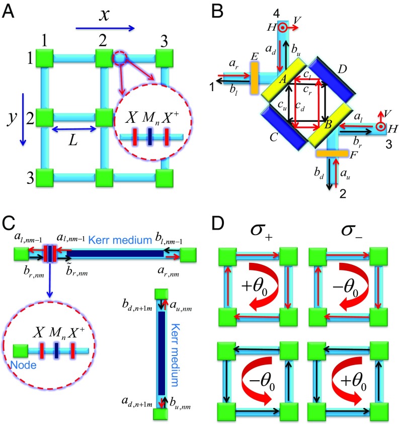
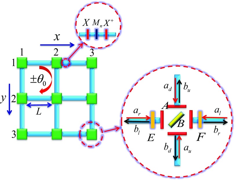
Fig. 1. Scheme of our optical network. (A) The planar network. (B) A node connects horizontal and vertical links. Here, ar,u,l,d and br,u,l,d denote the input and output amplitudes, and cr,u,l,d denotes the amplitudes in the cavity. The horizontal and vertical polarizations (H,V) in fibers are shown by the red circles and arrows. (C) The horizontal and vertical links with the Kerr medium and birefringent elements, where the Kerr medium is put on the right-hand side of three birefringent elements in the horizontal link, where the birefringent elements are assumed to have no Kerr nonlinearity (χ=0). From left to right, the three birefringent elements are described by the Jones matrices X=e^(iπσx/4), Mn=e^inθ0σz, and X^(†) in the linear polarization basis (H,V). (D) The σ+ polarized light acquires the phase θ0 (−θ0) by propagating (anti)clockwisely in each plaquette, while the σ− polarized light acquires the phase −θ0 (θ0) by propagating (anti)clockwisely in each plaquette.
Fig. 1. Scheme of our optical network. (A) The planar network. (B) A node connects horizontal and vertical links. Here, ar,u,l,d and br,u,l,d denote the input and output amplitudes, and cr,u,l,d denotes the amplitudes in the cavity. The horizontal and vertical polarizations (H,V) in fibers are shown by the red circles and arrows. (C) The horizontal and vertical links with the Kerr medium and birefringent elements, where the Kerr medium is put on the right-hand side of three birefringent elements in the horizontal link, where the birefringent elements are assumed to have no Kerr nonlinearity (χ=0). From left to right, the three birefringent elements are described by the Jones matrices X=e^(iπσx/4), Mn=e^inθ0σz, and X^(†) in the linear polarization basis (H,V). (D) The σ+ polarized light acquires the phase θ0 (−θ0) by propagating (anti)clockwisely in each plaquette, while the σ− polarized light acquires the phase −θ0 (θ0) by propagating (anti)clockwisely in each plaquette.CC BY-NC-ND · PubMed Central
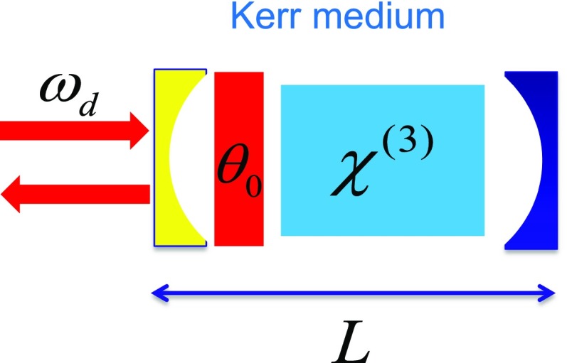
Fig. S1. A single Fabry–Perot cavity with Kerr nonlinearity and an anisotropic phase plate placed next to the left end mirror to mimic the horizontal link, where the driving field with frequency ωd is applied.
Fig. S1. A single Fabry–Perot cavity with Kerr nonlinearity and an anisotropic phase plate placed next to the left end mirror to mimic the horizontal link, where the driving field with frequency ωd is applied.CC BY-NC-ND · PubMed Central
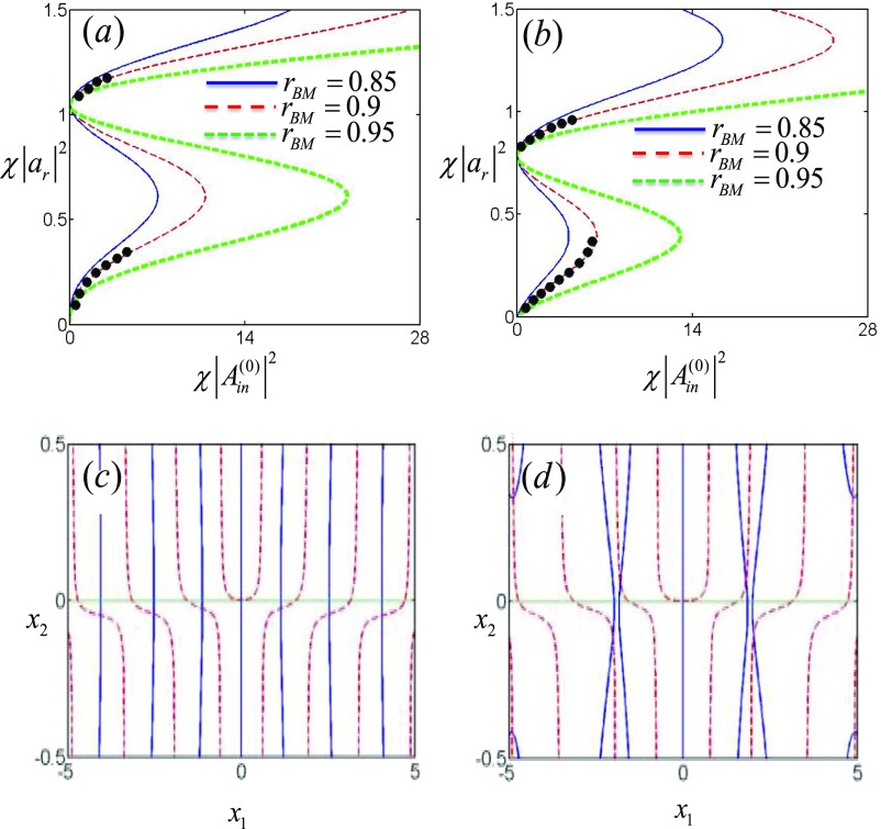
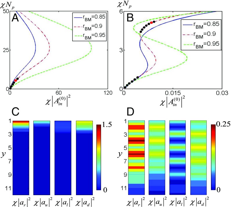
Fig. S2. Steady-state solutions and stability analysis, where L is taken as a unit. (A and B) The relation of the light intensity χ(|ar|)² in the cavity and the driving field intensity χ(|Ain⁽⁰⁾|)² in steady state for the driving frequencies ωd=3π/4 (A) and ωd=π/2 (B). Here, the stable regimes are marked by the black circles. The solid (blue), dashed (red), and dashed-dotted (green) curves denote the light intensities for rBM=0.85, 0.9, and 0.95, respectively. (C and D) For ωd=3π/4, the first and second equations in Eq. 27 are shown by the solid (blue) and dashed (red) curves, where χ(|Ain|)²=1, χ(|ar|)²=1.12 (C) and χ(|Ain|)²=5, χ(|ar|)²=1.21 (D).
Fig. S2. Steady-state solutions and stability analysis, where L is taken as a unit. (A and B) The relation of the light intensity χ(|ar|)² in the cavity and the driving field intensity χ(|Ain⁽⁰⁾|)² in steady state for the driving frequencies ωd=3π/4 (A) and ωd=π/2 (B). Here, the stable regimes are marked by the black circles. The solid (blue), dashed (red), and dashed-dotted (green) curves denote the light intensities for rBM=0.85, 0.9, and 0.95, respectively. (C and D) For ωd=3π/4, the first and second equations in Eq. 27 are shown by the solid (blue) and dashed (red) curves, where χ(|Ain|)²=1, χ(|ar|)²=1.12 (C) and χ(|Ain|)²=5, χ(|ar|)²=1.21 (D).CC BY-NC-ND · PubMed Central
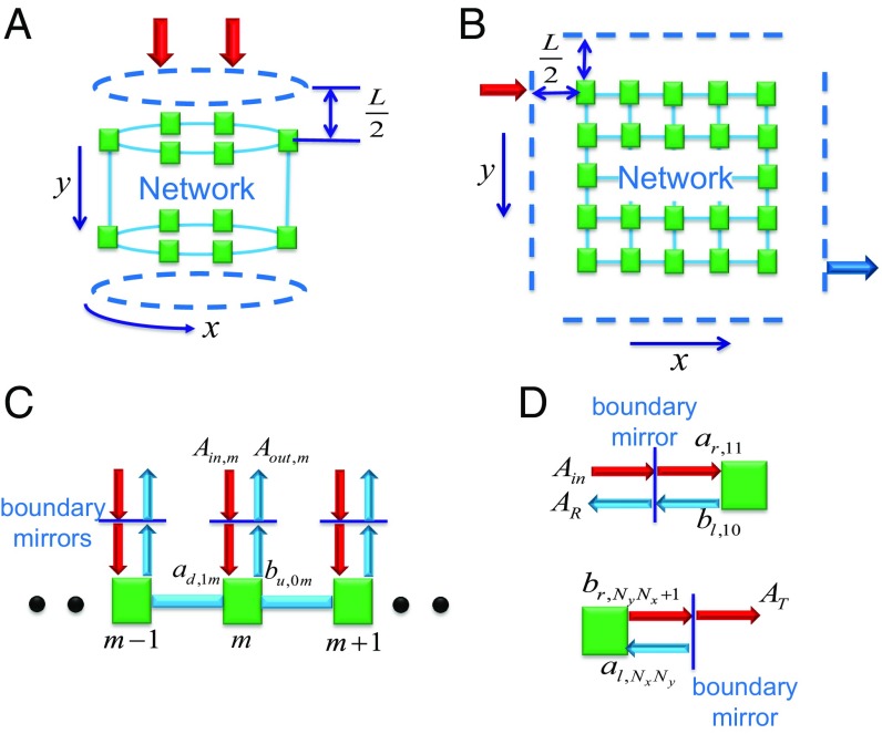
Fig. 2. Scheme for the boundary mirrors in the cylindrical and planar networks. (A and B) Perfect and partially transmissive mirrors are put along the boundaries of the cylindrical (A) and planar (B) networks. Here, the partially transmissive mirrors are placed along the top boundary in the cylindrical network and at the top left and bottom right corners in the planar network. The driving light (red arrows) is applied to generate the excitations and the transmitted light (blue arrow). (C) Driven cylindrical network through each of the partially transmissive mirrors on the top boundary. (D) Light reflection and transmission through the boundary mirrors next to the nodes (1,1) and (Ny,Nx) in the planar network (i.e., nodes in the top left and bottom right corners of the planar network).
Fig. 2. Scheme for the boundary mirrors in the cylindrical and planar networks. (A and B) Perfect and partially transmissive mirrors are put along the boundaries of the cylindrical (A) and planar (B) networks. Here, the partially transmissive mirrors are placed along the top boundary in the cylindrical network and at the top left and bottom right corners in the planar network. The driving light (red arrows) is applied to generate the excitations and the transmitted light (blue arrow). (C) Driven cylindrical network through each of the partially transmissive mirrors on the top boundary. (D) Light reflection and transmission through the boundary mirrors next to the nodes (1,1) and (Ny,Nx) in the planar network (i.e., nodes in the top left and bottom right corners of the planar network).CC BY-NC-ND · PubMed Central
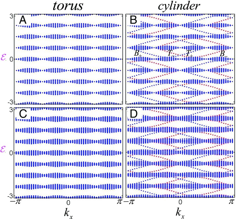
Fig. 3. The energy spectra in the torus and cylinder, where θ0=π/2, the network size is 48×48, and L is taken as a unit. Here, we use T± and B± to denote the σ± polarizations on the top and bottom boundaries, respectively. (A and B) The energy spectrum E in the torus (A) and cylinder (B) without phase randomness and losses of linear elements, where B and T denote the bottom and top boundaries, respectively. (C and D) The real part of the energy spectrum in the torus (C) and cylinder (D) with phase randomness and nonzero losses of linear elements.
Fig. 3. The energy spectra in the torus and cylinder, where θ0=π/2, the network size is 48×48, and L is taken as a unit. Here, we use T± and B± to denote the σ± polarizations on the top and bottom boundaries, respectively. (A and B) The energy spectrum E in the torus (A) and cylinder (B) without phase randomness and losses of linear elements, where B and T denote the bottom and top boundaries, respectively. (C and D) The real part of the energy spectrum in the torus (C) and cylinder (D) with phase randomness and nonzero losses of linear elements.CC BY-NC-ND · PubMed Central
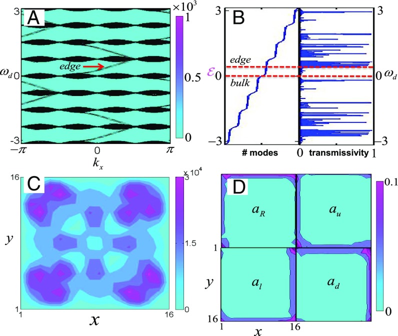
Fig. 4. Detection of topological properties, where θ0=π/2, rBM= 0.9, and L is taken as a unit. (A) For the cylindrical geometry, the contourplot of dδ0/dωd shows the eigenspectrum for the network of size 48× 48. (B) For the open plane of size 16× 16, the eigenspectrum for the closed network and the transmission spectrum. (C) The light intensity of the bulk mode under the σ+-polarized driving light. (D) The light intensities (|a(r,u,l,d)/Ain⁽⁰⁾|)² of the edge mode in the network under σ+-polarized driving light. From the right- (left-) and up- (down-)moving fields shown in the Top (Bottom) row, the chirality of the edge mode can be identified.
Fig. 4. Detection of topological properties, where θ0=π/2, rBM= 0.9, and L is taken as a unit. (A) For the cylindrical geometry, the contourplot of dδ0/dωd shows the eigenspectrum for the network of size 48× 48. (B) For the open plane of size 16× 16, the eigenspectrum for the closed network and the transmission spectrum. (C) The light intensity of the bulk mode under the σ+-polarized driving light. (D) The light intensities (|a(r,u,l,d)/Ain⁽⁰⁾|)² of the edge mode in the network under σ+-polarized driving light. From the right- (left-) and up- (down-)moving fields shown in the Top (Bottom) row, the chirality of the edge mode can be identified.CC BY-NC-ND · PubMed Central
Fig. S3. The new setup with tunable topological bandgaps. Here, the fiber is constructed similar to that in Fig. 1C of the main text, but now each node is built by four transmissive mirrors A with reflection amplitude rM and one beam-splitter B with reflection amplitude rbs. Two birefringent elements (E,F) in close proximity to the mirrors are described by the Jones matrix σz.
Fig. S3. The new setup with tunable topological bandgaps. Here, the fiber is constructed similar to that in Fig. 1C of the main text, but now each node is built by four transmissive mirrors A with reflection amplitude rM and one beam-splitter B with reflection amplitude rbs. Two birefringent elements (E,F) in close proximity to the mirrors are described by the Jones matrix σz.CC BY-NC-ND · PubMed Central
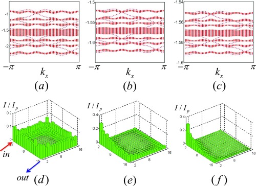
Fig. S4. (A–C) The energy spectra of the cylindrical network with 48×48 nodes for Rm=(|rM|)²={0.5,0.95,0.98}. (D–F) The light intensities of the steady edge modes in the open planar network with 16×16 nodes for Rm=(|rM|)²={0.5,0.95,0.98}, where the node and each birefringent element have 0.1% intrinsic loss.
Fig. S4. (A–C) The energy spectra of the cylindrical network with 48×48 nodes for Rm=(|rM|)²={0.5,0.95,0.98}. (D–F) The light intensities of the steady edge modes in the open planar network with 16×16 nodes for Rm=(|rM|)²={0.5,0.95,0.98}, where the node and each birefringent element have 0.1% intrinsic loss.CC BY-NC-ND · PubMed Central
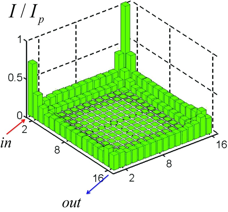
Fig. 5. The intensity of the steady edge mode in the open planar network, where the intrinsic loss is 0.1%, and Ip is the intensity of the pump field.
Fig. 5. The intensity of the steady edge mode in the open planar network, where the intrinsic loss is 0.1%, and Ip is the intensity of the pump field.CC BY-NC-ND · PubMed Central
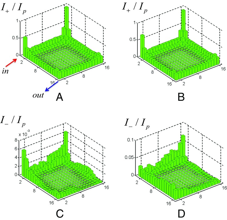
Fig. 6. A and C show the intensities I±/Ip of the σ±-polarized light in the network for δ,δ′∈[−0.05,0.05]; B and D show the intensities I±/Ip of the σ±-polarized light in the network for δ,δ′∈[−0.1,0.1].
Fig. 6. A and C show the intensities I±/Ip of the σ±-polarized light in the network for δ,δ′∈[−0.05,0.05]; B and D show the intensities I±/Ip of the σ±-polarized light in the network for δ,δ′∈[−0.1,0.1].CC BY-NC-ND · PubMed Central
Fig. 7. Light distributions of the nonlinear system in the cylinder, where the size is 24×12, θ0=π/2, kx=0.26, and L is taken as a unit. (A and B) The relation of the total intensity of (A) edge and (B) bulk modes in the network with different reflection indexes rBM and the input intensity of driving light with frequencies (A) ωd⁽¹⁾=0.22 and (B) ωd⁽²⁾=4.5×10⁻². (C and D) The stable internal intensities of (C) edge and (D) bulk modes for |χ|Np=5 and rBM=0.9 (red circles in A and B).
Fig. 7. Light distributions of the nonlinear system in the cylinder, where the size is 24×12, θ0=π/2, kx=0.26, and L is taken as a unit. (A and B) The relation of the total intensity of (A) edge and (B) bulk modes in the network with different reflection indexes rBM and the input intensity of driving light with frequencies (A) ωd⁽¹⁾=0.22 and (B) ωd⁽²⁾=4.5×10⁻². (C and D) The stable internal intensities of (C) edge and (D) bulk modes for |χ|Np=5 and rBM=0.9 (red circles in A and B).CC BY-NC-ND · PubMed Central
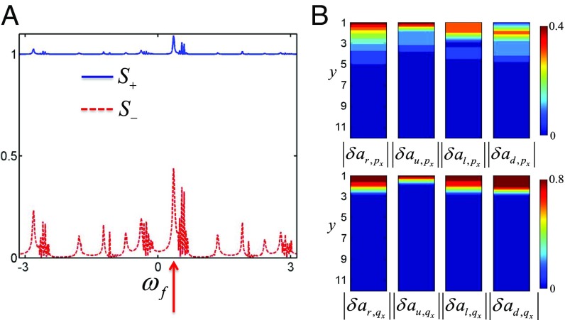
Fig. 8. Bogoliubov fluctuations in the cylinder, where the system size is 24×12, θ0=π/2. The amplitude |δAin⁽⁺⁾| of the probe light and L are taken as a unit. (A) The squeezing spectra of the probe field with the positive frequency, where the Bogoliubov fluctuations above the stable edge steady states are generated. (B) The distributions of Bogoliubov edge fluctuations above the stable edge steady states, where the Bogoliubov excitation has the frequency ωf=0.35, shown by the red arrow in A.
Fig. 8. Bogoliubov fluctuations in the cylinder, where the system size is 24×12, θ0=π/2. The amplitude |δAin⁽⁺⁾| of the probe light and L are taken as a unit. (A) The squeezing spectra of the probe field with the positive frequency, where the Bogoliubov fluctuations above the stable edge steady states are generated. (B) The distributions of Bogoliubov edge fluctuations above the stable edge steady states, where the Bogoliubov excitation has the frequency ωf=0.35, shown by the red arrow in A.CC BY-NC-ND · PubMed Central

Verification

Claims the paper makes

The claims and statistics of this paper haven’t been checked yet.

Run the check — free, no account needed. It reads the open-access text and checks the sources it cites.

A few free checks a day · papers already verified open instantly · results are public

Claims other papers make about this one

Each is checked against this paper’s own text: does it say what the citing paper says it does?

Self-check

Percentages, sums and reported differences re-computed from the paper’s own numbers.

The self-check needs the paper’s full text.

Citations

Cites

Research works printed but not linked: 52

  1. 10.1103/PhysRevLett.49.405 · DOI · Paper page
  2. 10.1103/PhysRevLett.61.2015 · DOI · Paper page
  3. 10.1103/RevModPhys.82.3045 · DOI · Paper page
  4. 10.1103/RevModPhys.83.1057 · DOI · Paper page
  5. 10.1103/PhysRevLett.95.226801 · DOI · Paper page
  6. 10.1126/science.1148047 · DOI · Paper page
  7. 10.1038/nature06843 · DOI · Paper page
  8. 10.1038/nphys1270 · DOI · Paper page
  9. 10.1126/science.1234414 · DOI · Paper page
  10. 10.1103/PhysRevLett.95.146802 · DOI · Paper page
  11. 10.1103/PhysRevB.74.195312 · DOI · Paper page
  12. 10.1142/S0217979292000840 · DOI
  13. 10.1103/PhysRevLett.50.1395 · DOI · Paper page
  14. 10.1016/0550-3213(91)90407-O · DOI
  15. 10.1038/nphoton.2013.274 · DOI · Paper page
  16. 10.1038/nature12066 · DOI · Paper page
  17. 10.1103/RevModPhys.83.1523 · DOI · Paper page
  18. 10.1103/PhysRevA.87.013606 · DOI
  19. 10.1103/PhysRevLett.100.013904 · DOI · Paper page
  20. 10.1038/nature08293 · DOI · Paper page
  21. 10.1038/nphoton.2012.236 · DOI · Paper page
  22. 10.1103/PhysRevA.92.053822 · DOI
  23. 10.1088/1367-2630/18/11/113029 · DOI
  24. 10.1038/ncomms10779 · DOI · Paper page
  25. 10.1103/PhysRevLett.108.206809 · DOI · Paper page
  26. 10.1038/nphys2063 · DOI · Paper page
  27. 10.1038/nmat3520 · DOI · Paper page
  28. 10.1103/PhysRevB.89.075113 · DOI
  29. W Hu, , Measurement of a topological edge invariant in a microwave network. Phys Rev X 5, 011012 (2015).
  30. 10.1103/PhysRevLett.76.4773 · DOI
  31. 10.1103/PhysRevLett.84.4184 · DOI · Paper page
  32. 10.1038/nmat4573 · DOI · Paper page
  33. R Bekenstein, J Nemirovsky, I Kaminer, M Segev, Shape-preserving accelerating electromagnetic wave packets in curved space. Phys Rev X 4, 011038 (2014).
  34. 10.1103/PhysRevA.94.021801 · DOI · Paper page
  35. 10.1103/PhysRevA.90.023813 · DOI
  36. 10.1103/PhysRevLett.117.143901 · DOI · Paper page
  37. 10.1364/OE.24.015631 · DOI · Paper page
  38. 10.1103/PhysRevB.93.020502 · DOI · Paper page
  39. 10.1016/B978-0-12-397023-7.00006-1 · DOI
  40. 10.1016/B978-0-12-369470-6.00002-2 · DOI
  41. 10.1364/JOSAB.15.000607 · DOI
  42. 10.1364/JOSAB.15.000617 · DOI
  43. 10.1016/0030-4018(81)90106-1 · DOI
  44. 10.1103/PhysRevB.39.3337 · DOI
  45. 10.1103/PhysRevB.14.2239 · DOI · Paper page
  46. MS Rudner, NH Lindner, E Berg, M Levin, Anomalous edge states and the bulk-edge correspondence for periodically driven two-dimensional systems. Phys Rev X 3, 031005 (2013).
  47. 10.1103/RevModPhys.85.299 · DOI · Paper page
  48. 10.1103/PhysRevB.93.085438 · DOI · Paper page
  49. 10.1103/PhysRevLett.108.206809 · DOI · Paper page
  50. 10.1103/PhysRevLett.111.243905 · DOI
  51. 10.1103/PhysRevA.88.063631 · DOI
  52. 10.1038/nature11298 · DOI · Paper page

Cited by

Sorted by citations

See all 20

Metadata

Authors
Shi, T., Kimble, H. J., & Cirac, J. I.
Affiliations
  • Max-Planck-Institut für Quantenoptik, 85748 Garching, Germany;
  • Norman Bridge Laboratory of Physics, California Institute of Technology, Pasadena, CA 91125
Venue
Proceedings of the National Academy of Sciences
Published
2017-10-10
Volume
114
Issue
43
ISSN
  • 0027-8424
  • 1091-6490
Cited by
20
References
4
Language
en

About these checks

Registry, retraction, Cites and statistics results are computed, not judged, with one exception: a printed reference that no index lists is read once by a model before it counts as a citation error. Claims are extracted by a model and kept only when their quote appears verbatim in the text; each cited source is then checked, with a model’s help, for whether it says what the claim relies on. Those verdicts can be wrong — read the claim’s quote and the cited source before relying on one.

Statistics and arithmetic are recomputed, not judged.

Confidence bands are shown only for fields calibrated on our annotated test set. None is calibrated yet, so no band is shown.

What counts as a claim ›How we measure confidence ›How we check this ›

Are you an author, or do you see a problem with this page? Request a review