Cited by 114Technology and Human Factors in Education and HealthModeling and Simulation SystemsScientific Computing and Data Management

The DOI matches its Crossref record; 18 of the 18 references it cites were found in a registry or an index.

A modular computational framework for medical digital twins

Open access
Masison, J., Beezley, J., Mei, Y., Ribeiro, HAL, Knapp, A. C., Sordo Vieira, L., Adhikari, B., Scindia, Y., Grauer, M., Helba, B., Schroeder, W., Mehrad, B., Laubenbacher, R.·2021·Proceedings of the National Academy of Sciences

Abstract

Significance: The digital twin paradigm holds great promise for medicine, even though many technical and scientific challenges remain to be overcome, most importantly the efficient integration of many heterogeneous component models. This is an unsolved problem even in industry. It has long been understood that such models need to be built in a modular fashion, connecting together component models of individual biological processes. In conventional implementations, however, the dependency structure of the modules reflects the dependencies among these processes, making it all but impossible to modify or expand the digital twin without breaking it. This paper presents a fundamental reorganization of the internal digital twin architecture into a hub-and-spokes design that completely circumvents this dependency problem.

Overview

The claims and statistics of this paper haven’t been checked yet.

Run the check — free, no account needed. It reads the open-access text and checks the sources it cites.

A few free checks a day · papers already verified open instantly · results are public

Integrity signals

Registry

Crossref · 10.1073/pnas.2024287118

Cites

18 of 18 references verified0 citation errors · 0 not checkable

Statistics

Figures

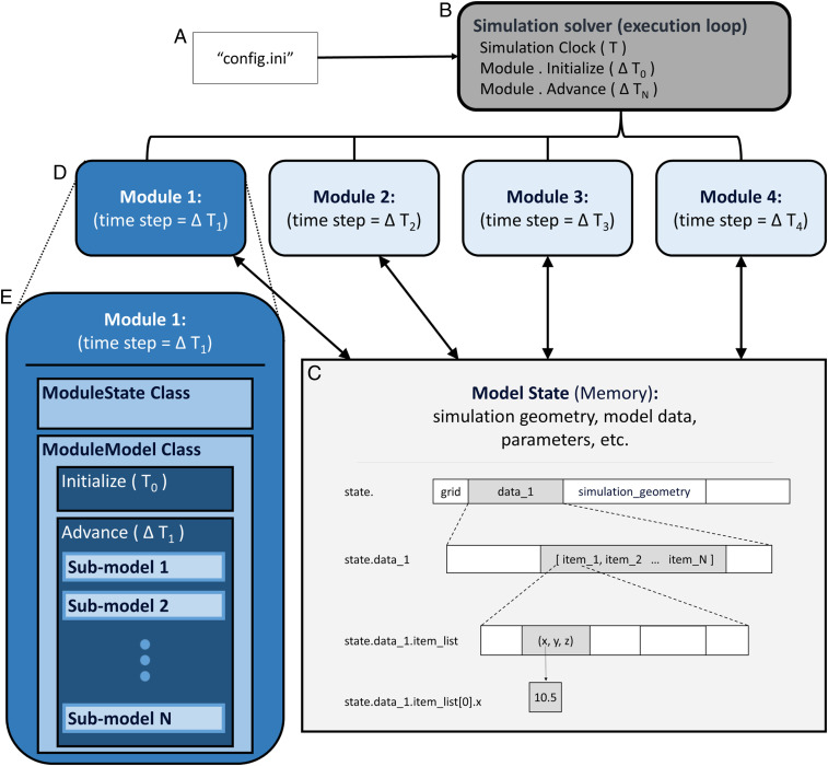
Fig. 1. Modular model components. The modular design implementation contains four components. (A) The runtime configuration file that contains all configuration and parameter settings for a given simulation run (“config.ini”). (B) A simulation solver that reads the configuration (config.ini) and constructs, initializes, and advances the simulation in time by executing each module according to its inherent time scale. (C) The model state contains all data describing the state of the model at a given point in time, including any physical space geometry, and states of model objects. In this example, the model includes a spatial component. The model state is a contiguous block of memory as shown by the partitioned rectangle, with the hierarchical Python-referencing syntax shown to the left of the representation. (D) Each module consists of a computational model that takes all input data from the model state and stores none itself. (E) These modules extend classes provided as part of the simulation framework, “ModuleState” and “ModuleModel,” which handle the connection to the simulation solver and model state access, so the developer only needs to consider the biological additions to the model. Extending the ModuleState results in the fields defined in the extending class being appended to the model state. The “initialize” and “advance” functions in the ModuleModel extension will be called by the simulation solver, so the module can participate in the simulation.
Fig. 1. Modular model components. The modular design implementation contains four components. (A) The runtime configuration file that contains all configuration and parameter settings for a given simulation run (“config.ini”). (B) A simulation solver that reads the configuration (config.ini) and constructs, initializes, and advances the simulation in time by executing each module according to its inherent time scale. (C) The model state contains all data describing the state of the model at a given point in time, including any physical space geometry, and states of model objects. In this example, the model includes a spatial component. The model state is a contiguous block of memory as shown by the partitioned rectangle, with the hierarchical Python-referencing syntax shown to the left of the representation. (D) Each module consists of a computational model that takes all input data from the model state and stores none itself. (E) These modules extend classes provided as part of the simulation framework, “ModuleState” and “ModuleModel,” which handle the connection to the simulation solver and model state access, so the developer only needs to consider the biological additions to the model. Extending the ModuleState results in the fields defined in the extending class being appended to the model state. The “initialize” and “advance” functions in the ModuleModel extension will be called by the simulation solver, so the module can participate in the simulation.CC BY · PubMed Central
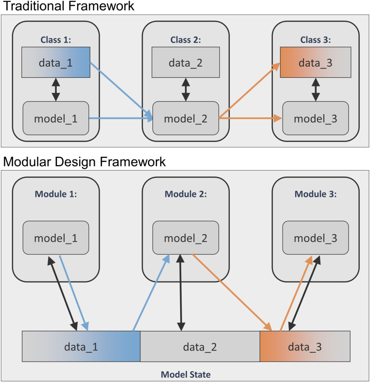
Fig. 2. Modular design framework enhancements over conventional model structure. In this simplified scenario, a model consists of three generic processes with dependencies. In both implementations, processes are separated into three distinct representations, modeled by functions (model_1, model_2, and model_3) that update data (data_1, data_2, and data_3) at each time step, with interactions indicated by arrows. In the above example, process 1 is intertwined with process 2 and process 2 with process 3. While the traditional architecture (Top) results in Class_2 depending on Class_1 (via model_2 depending on the Class 1 model and data API), the modular architecture (Bottom) results in Module_2 relying only on a subset of the global data defined by Module_1’s ModuleState (blue data_1). In contrast to the failure to run if model_1 changes in the traditional case, Module_1’s submodel (model_1) can change independently of the ModuleState (data_1) and preserve the validity of the Module_2 model (model_2). In the general situation, in which there is a new state that needs to be added to the module’s ModuleState (1) to support such submodel changes, this will likewise leave the other module (2) unaffected. If there are parts of the ModuleState (1) to be removed, this is the one case that could require alteration of other modules (2). However, in this case, regardless of the design, removal of a biological interaction demands that both classes involved be altered. Likewise, if new biology is added affecting multiple classes, both designs require changes to their models and inputs and outputs.
Fig. 2. Modular design framework enhancements over conventional model structure. In this simplified scenario, a model consists of three generic processes with dependencies. In both implementations, processes are separated into three distinct representations, modeled by functions (model_1, model_2, and model_3) that update data (data_1, data_2, and data_3) at each time step, with interactions indicated by arrows. In the above example, process 1 is intertwined with process 2 and process 2 with process 3. While the traditional architecture (Top) results in Class_2 depending on Class_1 (via model_2 depending on the Class 1 model and data API), the modular architecture (Bottom) results in Module_2 relying only on a subset of the global data defined by Module_1’s ModuleState (blue data_1). In contrast to the failure to run if model_1 changes in the traditional case, Module_1’s submodel (model_1) can change independently of the ModuleState (data_1) and preserve the validity of the Module_2 model (model_2). In the general situation, in which there is a new state that needs to be added to the module’s ModuleState (1) to support such submodel changes, this will likewise leave the other module (2) unaffected. If there are parts of the ModuleState (1) to be removed, this is the one case that could require alteration of other modules (2). However, in this case, regardless of the design, removal of a biological interaction demands that both classes involved be altered. Likewise, if new biology is added affecting multiple classes, both designs require changes to their models and inputs and outputs.CC BY · PubMed Central
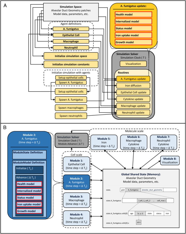
Fig. 3. Comparison between modular and conventional model implementation. Dependencies between components derived from source code and written description in the absence of code are outlined. (A) NetLogo model. An object-oriented model with a high level of interconnectedness among components. (B) Modular design structure. A hub-and-spoke model in which modules (spokes) interact directly only with the shared global state (the hub).
Fig. 3. Comparison between modular and conventional model implementation. Dependencies between components derived from source code and written description in the absence of code are outlined. (A) NetLogo model. An object-oriented model with a high level of interconnectedness among components. (B) Modular design structure. A hub-and-spoke model in which modules (spokes) interact directly only with the shared global state (the hub).CC BY · PubMed Central
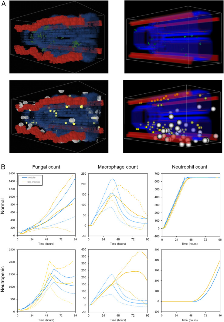
Fig. 4. (A) Simulation space. Both implementations (nonmodular left and modular right) share a similar simulation space. Both have a pair of alveolar ducts lined by epithelium branching from a single-source duct (where fungal cells lodge and germinate; green spheres in top row) and four blood vessels that run across the space parallel to the duct. The blood vessels are the source of recruited macrophages (white spheres), and neutrophils (yellow circles) are recruited (bottom row). The remaining space is filled with nonspecific interstitial tissue. (B) Simulation results. The panels show the results of both the modular (blue) and nonmodular (yellow) simulations for fungal cell count, macrophage cell count, and neutrophil cell count in both the normal immune response (Top) and neutropenic immune response (Bottom). Since both models are stochastic, they were simulated multiple times, beginning with the same initialization, and we have plotted averages and SDs. In the panels, the solid line is the mean, the long dashed line is one SD above the mean, and the short dashed line is one SD below the mean for 200 simulations. The figures were created using the code and configuration from release “version 0.1.1.”
Fig. 4. (A) Simulation space. Both implementations (nonmodular left and modular right) share a similar simulation space. Both have a pair of alveolar ducts lined by epithelium branching from a single-source duct (where fungal cells lodge and germinate; green spheres in top row) and four blood vessels that run across the space parallel to the duct. The blood vessels are the source of recruited macrophages (white spheres), and neutrophils (yellow circles) are recruited (bottom row). The remaining space is filled with nonspecific interstitial tissue. (B) Simulation results. The panels show the results of both the modular (blue) and nonmodular (yellow) simulations for fungal cell count, macrophage cell count, and neutrophil cell count in both the normal immune response (Top) and neutropenic immune response (Bottom). Since both models are stochastic, they were simulated multiple times, beginning with the same initialization, and we have plotted averages and SDs. In the panels, the solid line is the mean, the long dashed line is one SD above the mean, and the short dashed line is one SD below the mean for 200 simulations. The figures were created using the code and configuration from release “version 0.1.1.”CC BY · PubMed Central
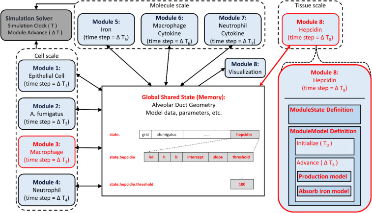
Fig. 5. Adding a module to the model. To add the process of hepcidin regulation of macrophage iron handling to the existing model, we only need to create or change the components highlighted in red; a new module (Module 8: Hepcidin) is added with a ModuleState and ModuleModel definition, a new section in the configuration file, and any changes to the existing module’s models (Macrophage) required by the incorporation of a new biological factor. Using the ModuleState and ModuleModel superclasses makes this process of addition very simple, as the only new code is related to the new hepcidin biology, with the connection to the rest of the simulation handled by the components of the modular framework. The new code will exist in three places: 1) in a listing of the new model state under the extension of the ModuleState, 2) in the implementation of the “Production model” and “Absorb iron model” within the advance function, and 3) in the implementation of the initialize function for reading the appropriate values from the configuration file and any other required action for initialization. During initialization and time stepping, the simulation framework will ensure that the new module state is appended and the new module receives the full model state to run its models at each time step.
Fig. 5. Adding a module to the model. To add the process of hepcidin regulation of macrophage iron handling to the existing model, we only need to create or change the components highlighted in red; a new module (Module 8: Hepcidin) is added with a ModuleState and ModuleModel definition, a new section in the configuration file, and any changes to the existing module’s models (Macrophage) required by the incorporation of a new biological factor. Using the ModuleState and ModuleModel superclasses makes this process of addition very simple, as the only new code is related to the new hepcidin biology, with the connection to the rest of the simulation handled by the components of the modular framework. The new code will exist in three places: 1) in a listing of the new model state under the extension of the ModuleState, 2) in the implementation of the “Production model” and “Absorb iron model” within the advance function, and 3) in the implementation of the initialize function for reading the appropriate values from the configuration file and any other required action for initialization. During initialization and time stepping, the simulation framework will ensure that the new module state is appended and the new module receives the full model state to run its models at each time step.CC BY · PubMed Central
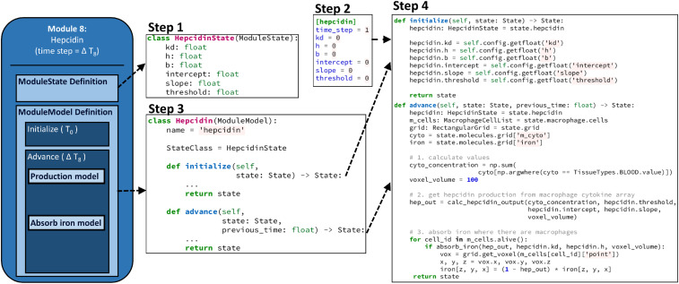
Fig. 6. Addition of the Hepcidin module. 1) The hepcidin module must define a subclass of ModuleState, called here “HepcidinState.” Below, all the data related to the ModuleState (six relevant variables) are simply floating-point numbers, but, as noted above, the type of data could also be integers, Boolean, strings, and NumPy arrays of these types. 2) The config.ini file must be altered. The path of the new module file “hepcidin.py” (simulation\modules\hepcidin.py) is added to the modules field under the simulation heading, in the form simulation.modules.hepcidin. Hepcidin, in which Hepcidin is the class extending ModuleModel to be coded in the next step. All the parameters relevant to the hepcidin module are given a value under a new “hepcidin” heading. This section must also include a time_step field, which indicates the period over which the module is to be updated. 3) The third necessary step is to code a subclass of “ModuleModel,” called here “Hepcidin.” Setting values of the “name” and StateClass field are required. 4) The last step is to code the model by implementing initialize() and/or advance() functions. The new hepcidin module will have six parameters, each of which are initialized based on the values provided in the configuration file in the initialize function. Within the “advance” function, all submodels related to the module will be executed. In this example, this includes calculating values, getting a hepcidin number from the macrophage cytokine level, and absorbing iron where biologically indicated.
Fig. 6. Addition of the Hepcidin module. 1) The hepcidin module must define a subclass of ModuleState, called here “HepcidinState.” Below, all the data related to the ModuleState (six relevant variables) are simply floating-point numbers, but, as noted above, the type of data could also be integers, Boolean, strings, and NumPy arrays of these types. 2) The config.ini file must be altered. The path of the new module file “hepcidin.py” (simulation\modules\hepcidin.py) is added to the modules field under the simulation heading, in the form simulation.modules.hepcidin. Hepcidin, in which Hepcidin is the class extending ModuleModel to be coded in the next step. All the parameters relevant to the hepcidin module are given a value under a new “hepcidin” heading. This section must also include a time_step field, which indicates the period over which the module is to be updated. 3) The third necessary step is to code a subclass of “ModuleModel,” called here “Hepcidin.” Setting values of the “name” and StateClass field are required. 4) The last step is to code the model by implementing initialize() and/or advance() functions. The new hepcidin module will have six parameters, each of which are initialized based on the values provided in the configuration file in the initialize function. Within the “advance” function, all submodels related to the module will be executed. In this example, this includes calculating values, getting a hepcidin number from the macrophage cytokine level, and absorbing iron where biologically indicated.CC BY · PubMed Central

Verification

Claims the paper makes

The claims and statistics of this paper haven’t been checked yet.

Run the check — free, no account needed. It reads the open-access text and checks the sources it cites.

A few free checks a day · papers already verified open instantly · results are public

Claims other papers make about this one

Each is checked against this paper’s own text: does it say what the citing paper says it does?

Self-check

Percentages, sums and reported differences re-computed from the paper’s own numbers.

The self-check needs the paper’s full text.

Citations

Cites

Show all 18 references

Cited by

Sorted by citations

Items 101–114 of 114

Metadata

Authors
Masison, J., Beezley, J., Mei, Y., Ribeiro, H., Knapp, A. C., Sordo Vieira, L., Adhikari, B., Scindia, Y., Grauer, M., Helba, B., Schroeder, W., Mehrad, B., & Laubenbacher, R.
Affiliations
  • UConn Health (US)
  • Kitware (United States) (US)
  • University of Michigan (US)
  • Department of Medicine, University of Florida, Gainesville, FL 32611
  • University of Florida (US)
Corresponding author
Laubenbacher, R.
Venue
Proceedings of the National Academy of Sciences
Published
2021-05-10
Volume
118
Issue
20
ISSN
  • 0027-8424 (ISSN-L)
  • 1091-6490
OpenAlex
W3163235749
Cited by
98
References
18
Citations by year
2026: 14 · 2025: 25 · 2024: 18 · 2023: 19 · 2022: 19 · 2021: 3
FWCI
16.25
Type
journal article
Language
en
Open access
Locations
  • Proceedings of the National Academy of Sciences (publishedVersion, cc-by)
  • PubMed Central (publishedVersion, cc-by)
  • PubMed (publishedVersion)
Funders
  • HHS | NIH | National Institute of Biomedical Imaging and Bioengineering (1U01EB024501-01)
  • HHS | NIH | National Institute of Allergy and Infectious Diseases (1 R01AI135128-01)
  • HHS | NIH | National Institute of General Medical Sciences (1R01GM127909-01)
  • HHS | NIH | National Institute of Dental and Craniofacial Research (T-90DE021989)
  • American Heart Association (18TPA34170486)
Topics
  • Health Sciences › Medicine › Public Health, Environmental and Occupational Health › Technology and Human Factors in Education and Health
  • Physical Sciences › Mathematics › Modeling and Simulation › Modeling and Simulation Systems
  • Social Sciences › Decision Sciences › Information Systems and Management › Scientific Computing and Data Management
Keywords
medical digital twins, modular software platform, precision medicine, patient-specific disease modeling, model integration, data-driven modeling, mechanistic modeling, open source software, respiratory fungal infection, personalized treatment
MeSH terms
Algorithms, Animals, Antifungal Agents, Aspergillosis, Aspergillus fumigatus, Humans, Software, Spores, Fungal, Computational Biology, Precision Medicine, Patient-Specific Modeling

About these checks

Registry, retraction, Cites and statistics results are computed, not judged, with one exception: a printed reference that no index lists is read once by a model before it counts as a citation error. Claims are extracted by a model and kept only when their quote appears verbatim in the text; each cited source is then checked, with a model’s help, for whether it says what the claim relies on. Those verdicts can be wrong — read the claim’s quote and the cited source before relying on one.

Statistics and arithmetic are recomputed, not judged.

Confidence bands are shown only for fields calibrated on our annotated test set. None is calibrated yet, so no band is shown.

What counts as a claim ›How we measure confidence ›How we check this ›

Are you an author, or do you see a problem with this page? Request a review