Student or educator? Sign up with your school email and get 6 months of Pro free.
PreprintCited by 1Angiogenesis and VEGF in CancerMathematical Biology Tumor GrowthGene Regulatory Network Analysis

The DOI matches its Crossref record; 1 of the 1 references it cites were found in a registry or an index.

Mechanistic computational modeling of sFLT1 secretion dynamics

Open access
Gill, Amy, Kinghorn, Karina, Bautch, Victoria L., Mac Gabhann, Feilim·2025·PLoS Computational Biology

Preprint — published as 10.1371/journal.pcbi.1013324 · Paper page

Abstract

Constitutively secreted by endothelial cells, soluble FLT1 (sFLT1 or sVEGFR1) binds and sequesters extracellular vascular endothelial growth factors (VEGF), thereby reducing VEGF binding to VEGF receptor tyrosine kinases and their downstream signaling. In doing so, sFLT1 plays an important role in vascular development and in the patterning of new blood vessels in angiogenesis. Here, we develop multiple mechanistic models of sFLT1 secretion and identify a minimal mechanistic model that recapitulates key qualitative and quantitative features of temporal experimental datasets of sFLT1 secretion from multiple studies. We show that the experimental data on sFLT1 secretion is best represented by a delay differential equation (DDE) system including a maturation term, reflecting the time required between synthesis and secretion. Using optimization to identify appropriate values for the key mechanistic parameters in the model, we show that two model parameters (extracellular degradation rate constant and maturation time) are very strongly constrained by the experimental data, and that the remaining parameters are related by two strongly constrained constants. Thus, only one degree of freedom remains, and measurements of the intracellular levels of sFLT1 would fix the remaining parameters. Comparison between simulation predictions and additional experimental data of the outcomes of chemical inhibitors and genetic perturbations suggest that intermediate values of the secretion rate constant best match the simulation with experiments, which would completely constrain the model. However, some of the inhibitors tested produce results that cannot be reproduced by the model simulations, suggesting that additional mechanisms not included here are required to explain those inhibitors. Overall, the model reproduces most available experimental data and suggests targets for further quantitative investigation of the sFLT1 system. Author Summary: Proteins that are typically found outside cells are initially made inside cells, and later secreted into extracellular space. Many of these secreted proteins have important functions outside the cell that are well-studied; however, usually much less is known about the pre-secretion life of these molecules. Many computational models only represent the extracellular versions of secreted proteins, reducing all production and secretion steps into a single modeled process. Here, we develop a mechanistic model of the production and secretion of a specific secreted protein, sFLT1, which inhibits blood vessel growth by acting as an extracellular sponge for another set of secreted proteins, the vascular endothelial growth factors. We compare several models to existing experimentally-measured sFLT1 data, and we show that the data are most simply explained by including a delay between intracellular sFLT1 production and sFLT1 transport or degradation. This is consistent with the biology of the cell’s secretory pathway, where immature proteins are gradually processed into mature forms over minutes to hours. Our approach could be incorporated into improved models for any pathway involving secreted proteins, including sFLT1-regulated models of blood vessel biology.

Overview

The claims and statistics of this paper haven’t been checked yet.

Run the check — free, no account needed. It reads the open-access text and checks the sources it cites.

A few free checks a day · papers already verified open instantly · results are public

Integrity signals

Registry

Crossref · 10.1101/2025.02.12.637983

Cites

1 of 1 references verified0 citation errors · 0 not checkable

Statistics

Figures

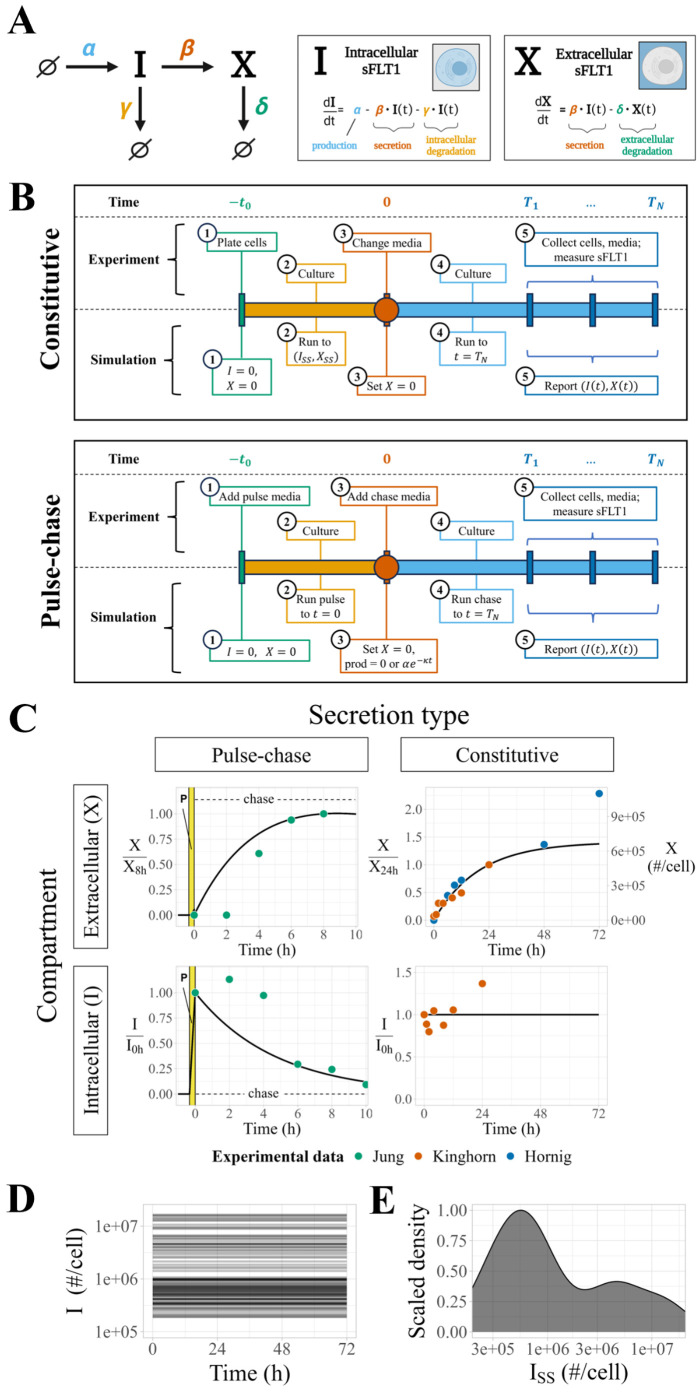
Fig 1 Modeling sFLT1 secretion with ordinary differential equations (ODEs). (A) Model of sFLT1 secretion dynamics describing the impact of production (rate α), secretion (rate constant β), intracellular degradation (γ), and extracellular degradation (δ) on the concentrations of intracellular (I) and extracellular (X) sFLT1 as a system of ordinary differential equations (ODEs). Created with BioRender.com. (B) Comparison of simulation (top row) and experimental (bottom row) approaches for studying sFLT1 secretion in the constitutive secretion scenario (left column) and pulse-chase secretion scenario (right column). (C) Simulated time courses (n = 100) of extracellular (X, top) and intracellular (I, bottom) sFLT1 secretion for pulse-chase (left) and constitutive (right) cases using the ODE model. X was normalized to its value at 8h (upper left) or 24h (upper right), while I was normalized to its value at 0h. The highlighted region (P) marks the 20-minute pulse. (D) Number of intracellular sFLT1 (I) molecules per cell over time and (E) distribution of steady state intracellular sFLT1 (ISS) during simulations of constitutive secretion using the ODE model.
Fig 1 Modeling sFLT1 secretion with ordinary differential equations (ODEs). (A) Model of sFLT1 secretion dynamics describing the impact of production (rate α), secretion (rate constant β), intracellular degradation (γ), and extracellular degradation (δ) on the concentrations of intracellular (I) and extracellular (X) sFLT1 as a system of ordinary differential equations (ODEs). Created with BioRender.com. (B) Comparison of simulation (top row) and experimental (bottom row) approaches for studying sFLT1 secretion in the constitutive secretion scenario (left column) and pulse-chase secretion scenario (right column). (C) Simulated time courses (n = 100) of extracellular (X, top) and intracellular (I, bottom) sFLT1 secretion for pulse-chase (left) and constitutive (right) cases using the ODE model. X was normalized to its value at 8h (upper left) or 24h (upper right), while I was normalized to its value at 0h. The highlighted region (P) marks the 20-minute pulse. (D) Number of intracellular sFLT1 (I) molecules per cell over time and (E) distribution of steady state intracellular sFLT1 (ISS) during simulations of constitutive secretion using the ODE model.CC BY · PubMed Central
Fig 2 Modeling sFLT1 secretion with delay differential equations (DDEs). (A) Model of sFLT1 secretion dynamics as a system of delay differential equations (DDEs), extending the ODE model (Fig 1A) with a fixed maturation delay (τ) affecting secretion and intracellular degradation processes. Created with Biorender.com. (B) Simulated time courses (n=594) of extracellular (X, top) and intracellular (I, bottom) sFLT1 secretion for pulse-chase (left) and constitutive (right) cases using the base DDE model. X was normalized to its value at 8h (upper left) or 24h (upper right), while I was normalized to its value at 0h. The highlighted region (P) marks the 20-minute pulse.
Fig 2 Modeling sFLT1 secretion with delay differential equations (DDEs). (A) Model of sFLT1 secretion dynamics as a system of delay differential equations (DDEs), extending the ODE model (Fig 1A) with a fixed maturation delay (τ) affecting secretion and intracellular degradation processes. Created with Biorender.com. (B) Simulated time courses (n=594) of extracellular (X, top) and intracellular (I, bottom) sFLT1 secretion for pulse-chase (left) and constitutive (right) cases using the base DDE model. X was normalized to its value at 8h (upper left) or 24h (upper right), while I was normalized to its value at 0h. The highlighted region (P) marks the 20-minute pulse.CC BY · PubMed Central
Fig 3 Comparing candidate models of sFLT1 secretion. (A) Structure of candidate model equations and equation term options for each process when present or absent in a given model. In the production decay term, the value of [chase] is 1 during the chase phase of pulse-chase simulations and 0 otherwise. (B) Top: Processes included (filled) or excluded (empty) in each model. ε: internalization, κ: production decay, τ: maturation delay. Middle: Cost (goodness of fit) of each model, defined as the sum of squared differences (SSD) between experimental data points and the lowest cost simulation of each model, with colors indicating the contribution of each experimental dataset. X: extracellular sFLT1, I: intracellular sFLT1. Bottom: Corrected Akaike Information Criterion (AICC) scores for each model. All models are fit to the same number of observations (n=26), while the number of parameters k varies by model. (C) Impact of additional processes on the best-fit cost of the candidate models. Model nodes (points) are plotted as minimum model cost versus number of parameters k. Edges (arrows) represent transitions between candidate model structures by adding the labeled process (τ (maturation delay): pink arrows, κ (production decay): blue arrows, ε (internalization): gray arrows. The vertical height of each arrow represents the decrease in cost from adding the labeled process to a given model.
Fig 3 Comparing candidate models of sFLT1 secretion. (A) Structure of candidate model equations and equation term options for each process when present or absent in a given model. In the production decay term, the value of [chase] is 1 during the chase phase of pulse-chase simulations and 0 otherwise. (B) Top: Processes included (filled) or excluded (empty) in each model. ε: internalization, κ: production decay, τ: maturation delay. Middle: Cost (goodness of fit) of each model, defined as the sum of squared differences (SSD) between experimental data points and the lowest cost simulation of each model, with colors indicating the contribution of each experimental dataset. X: extracellular sFLT1, I: intracellular sFLT1. Bottom: Corrected Akaike Information Criterion (AICC) scores for each model. All models are fit to the same number of observations (n=26), while the number of parameters k varies by model. (C) Impact of additional processes on the best-fit cost of the candidate models. Model nodes (points) are plotted as minimum model cost versus number of parameters k. Edges (arrows) represent transitions between candidate model structures by adding the labeled process (τ (maturation delay): pink arrows, κ (production decay): blue arrows, ε (internalization): gray arrows. The vertical height of each arrow represents the decrease in cost from adding the labeled process to a given model.CC BY · PubMed Central
Fig 4 Properties of optimized parameter sets from the DDE model of sFLT1 secretion. (A) Distributions of initial (yellow) and optimized (black) model parameter values for the delay differential equation model after filtering for low-cost fits (n = 594). Y axes are normalized such that each distribution has a maximum density of 1. (B) Correlations between α, β, and γ values in optimized parameter sets. Each point represents the observed values of the listed parameters in a single run of the delay differential equation model after filtering for low-cost fits (n = 594). (C) Distributions of initial (yellow) and optimized (black) values of calculated compound parameters c1 = αβ and c2 = β + γ for the delay differential equation model after filtering for low-cost fits (n = 594). (D-G) Correlation between intracellular steady state sFLT1 (ISS) and (D) α/(β + γ), (E) α, (F) β, (G) γ. Dashed lines indicate theoretical bounds (min(ISS) =c1/c2², min(α) =c1/c2, min(β) = min(γ) = 0, max(β) = max(γ) = 0; see S2 Text. Bounds and highlighted trendlines are calculated using median values of c1 and c2 (Table 1).
Fig 4 Properties of optimized parameter sets from the DDE model of sFLT1 secretion. (A) Distributions of initial (yellow) and optimized (black) model parameter values for the delay differential equation model after filtering for low-cost fits (n = 594). Y axes are normalized such that each distribution has a maximum density of 1. (B) Correlations between α, β, and γ values in optimized parameter sets. Each point represents the observed values of the listed parameters in a single run of the delay differential equation model after filtering for low-cost fits (n = 594). (C) Distributions of initial (yellow) and optimized (black) values of calculated compound parameters c1 = αβ and c2 = β + γ for the delay differential equation model after filtering for low-cost fits (n = 594). (D-G) Correlation between intracellular steady state sFLT1 (ISS) and (D) α/(β + γ), (E) α, (F) β, (G) γ. Dashed lines indicate theoretical bounds (min(ISS) =c1/c2², min(α) =c1/c2, min(β) = min(γ) = 0, max(β) = max(γ) = 0; see S2 Text. Bounds and highlighted trendlines are calculated using median values of c1 and c2 (Table 1).CC BY · PubMed Central
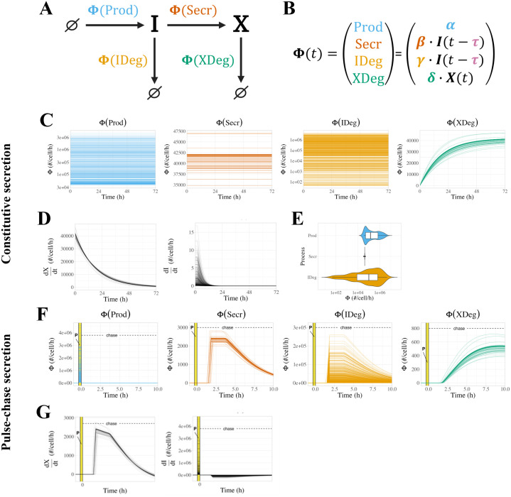
Fig 5 Analysis of simulated sFLT1 kinetic process fluxes. (A) Reaction network graph showing process fluxes (Φ). (B) Equations for process fluxes. (C) Process fluxes over time during simulation of constitutive sFLT1 secretion. (D) Rates of change of extracellular sFLT1 (dX/dt = Φ(Secr) − Φ(XDeg)) and intracellular sFLT1 (dI/dt = Φ(Prod) − Φ(Secr) − Φ(IDeg)) during constitutive secretion. (E) Constitutive flux distributions for time-constant processes. (F) Process fluxes over time during simulation of pulse-chase sFLT1 secretion. (G) Rates of change of extracellular and intracellular sFLT1 during pulse-chase secretion. In C, D, F, and G, each line represents a different optimized parameter set. Prod = production, Secr = secretion, IDeg = intracellular degradation, XDeg = extracellular degradation.
Fig 5 Analysis of simulated sFLT1 kinetic process fluxes. (A) Reaction network graph showing process fluxes (Φ). (B) Equations for process fluxes. (C) Process fluxes over time during simulation of constitutive sFLT1 secretion. (D) Rates of change of extracellular sFLT1 (dX/dt = Φ(Secr) − Φ(XDeg)) and intracellular sFLT1 (dI/dt = Φ(Prod) − Φ(Secr) − Φ(IDeg)) during constitutive secretion. (E) Constitutive flux distributions for time-constant processes. (F) Process fluxes over time during simulation of pulse-chase sFLT1 secretion. (G) Rates of change of extracellular and intracellular sFLT1 during pulse-chase secretion. In C, D, F, and G, each line represents a different optimized parameter set. Prod = production, Secr = secretion, IDeg = intracellular degradation, XDeg = extracellular degradation.CC BY · PubMed Central
Fig 6 Local and global univariate sensitivity analysis of the sFLT1 secretion DDE model. (A) Relative sensitivity of sFLT1 secretion output variables to local changes in input parameters during simulation of constitutive secretion. The base case is the median parameter set, and all other cells represent the observed fractional increase in the output variable per fractional increase in the parameter. X72h: extracellular sFLT1 after 72 hours; I72h: intracellular sFLT1 after 72 hours; T50_X: time to half-steady-state for extracellular sFLT1. (B) Global univariate sensitivity analysis of extracellular and intracellular sFLT1 showing the effect of multiplying each input parameter by a scaling factor during constitutive secretion. The base case (scaling factor 1) is the median parameter set from the optimized parameter sets (Table 1).
Fig 6 Local and global univariate sensitivity analysis of the sFLT1 secretion DDE model. (A) Relative sensitivity of sFLT1 secretion output variables to local changes in input parameters during simulation of constitutive secretion. The base case is the median parameter set, and all other cells represent the observed fractional increase in the output variable per fractional increase in the parameter. X72h: extracellular sFLT1 after 72 hours; I72h: intracellular sFLT1 after 72 hours; T50_X: time to half-steady-state for extracellular sFLT1. (B) Global univariate sensitivity analysis of extracellular and intracellular sFLT1 showing the effect of multiplying each input parameter by a scaling factor during constitutive secretion. The base case (scaling factor 1) is the median parameter set from the optimized parameter sets (Table 1).CC BY · PubMed Central
Fig 7 Simulated chemical inhibition and genetic downregulation of sFLT1 secretion. (A) Simulation timeline schematic for chemical inhibition (top) and genetic downregulation (bottom) of constitutive secretion. p=p′ represents change of parameter values to apply inhibitor effect. (B) Effects of chemical inhibition of individual parameters by 90% on extracellular sFLT1 (X) and intracellular sFLT1 (I) at 18h and 72h, expressed as log2 fold changes relative to the control (uninhibited) case. (C) Time courses for absolute concentrations of extracellular (X) and intracellular (I) sFLT1 with 90% chemical inhibition of each parameter. The impact of inhibiting each process is how different each line is from the prediction of the median, unmodified parameter set (black line). The inset magnifies the trend for inhibition of α. Black points, experimental ELISA data for the uninhibited case [29]. (D) Annotated curves for chemical inhibition of β (red) and γ (orange) reproduced from (C). Horizontal lines indicate experimentally observed relative changes in extracellular (X18h) and intracellular (I18h) sFLT1 18 hours after drug addition. Vertical lines indicate the fraction inhibition of the target parameter required to reproduce experimental results. (E) Effects of genetic downregulation of individual parameters by 90%, as described in (B). (F) Time courses for absolute concentrations of extracellular (X) and intracellular (I) sFLT1 with 90% genetic downregulation of each parameter, as described in (C). (G) Annotated curves for genetic downregulation of β (red) and γ (orange), as described in (D).
Fig 7 Simulated chemical inhibition and genetic downregulation of sFLT1 secretion. (A) Simulation timeline schematic for chemical inhibition (top) and genetic downregulation (bottom) of constitutive secretion. p=p′ represents change of parameter values to apply inhibitor effect. (B) Effects of chemical inhibition of individual parameters by 90% on extracellular sFLT1 (X) and intracellular sFLT1 (I) at 18h and 72h, expressed as log2 fold changes relative to the control (uninhibited) case. (C) Time courses for absolute concentrations of extracellular (X) and intracellular (I) sFLT1 with 90% chemical inhibition of each parameter. The impact of inhibiting each process is how different each line is from the prediction of the median, unmodified parameter set (black line). The inset magnifies the trend for inhibition of α. Black points, experimental ELISA data for the uninhibited case [29]. (D) Annotated curves for chemical inhibition of β (red) and γ (orange) reproduced from (C). Horizontal lines indicate experimentally observed relative changes in extracellular (X18h) and intracellular (I18h) sFLT1 18 hours after drug addition. Vertical lines indicate the fraction inhibition of the target parameter required to reproduce experimental results. (E) Effects of genetic downregulation of individual parameters by 90%, as described in (B). (F) Time courses for absolute concentrations of extracellular (X) and intracellular (I) sFLT1 with 90% genetic downregulation of each parameter, as described in (C). (G) Annotated curves for genetic downregulation of β (red) and γ (orange), as described in (D).CC BY · PubMed Central
Fig 8 Simulating chemical and genetic inhibition of sFLT1 secretion from different initial parameter sets. (A) Annotated curves for chemical inhibition of β (secretion, first 3 columns) and γ (intracellular degradation, rightmost column) at 18 hours. Horizontal lines indicate experimentally observed relative changes in extracellular (X18h) and intracellular (I18h) sFLT1 18 hours after addition of brefeldin, chlorpromazine, TATNSF700, or chloroquine. Colored vertical lines mark the fraction inhibition required to match the observed change in sFLT1 when starting from the parameter set with the matching β value. (B) Annotated curves for genetic inhibition of β (secretion rate constant) at 18 hours post media change. Horizontal lines indicate experimentally observed relative changes in extracellular (X18h) and intracellular (I18h) sFLT1 after 18 hours after media change in cells transfected with siRNA targeting the listed secretion-linked protein 48 hours previously [13]. Colored vertical lines mark the fraction inhibition required to match the observed change in sFLT1 when starting from the parameter set with the matching β value.
Fig 8 Simulating chemical and genetic inhibition of sFLT1 secretion from different initial parameter sets. (A) Annotated curves for chemical inhibition of β (secretion, first 3 columns) and γ (intracellular degradation, rightmost column) at 18 hours. Horizontal lines indicate experimentally observed relative changes in extracellular (X18h) and intracellular (I18h) sFLT1 18 hours after addition of brefeldin, chlorpromazine, TATNSF700, or chloroquine. Colored vertical lines mark the fraction inhibition required to match the observed change in sFLT1 when starting from the parameter set with the matching β value. (B) Annotated curves for genetic inhibition of β (secretion rate constant) at 18 hours post media change. Horizontal lines indicate experimentally observed relative changes in extracellular (X18h) and intracellular (I18h) sFLT1 after 18 hours after media change in cells transfected with siRNA targeting the listed secretion-linked protein 48 hours previously [13]. Colored vertical lines mark the fraction inhibition required to match the observed change in sFLT1 when starting from the parameter set with the matching β value.CC BY · PubMed Central

Verification

Claims the paper makes

The claims and statistics of this paper haven’t been checked yet.

Run the check — free, no account needed. It reads the open-access text and checks the sources it cites.

A few free checks a day · papers already verified open instantly · results are public

Self-check

Percentages, sums and reported differences re-computed from the paper’s own numbers.

The self-check needs the paper’s full text.

Citations

Cites

Research works printed but not linked: 55

  1. 10.1126/science.1260419 · DOI · Paper page
  2. 10.1126/science.1096303 · DOI
  3. 10.1126/scisignal.aaz0274 · DOI · Paper page
  4. 10.1016/S0962-8924(97)01197-5 · DOI
  5. 10.1242/jcs.258564 · DOI
  6. 10.1038/onc.2013.1 · DOI
  7. 10.1016/S0021-9258(18)37798-6 · DOI
  8. 10.1016/j.yexcr.2008.12.020 · DOI
  9. 10.1038/nrm2748 · DOI · Paper page
  10. 10.1016/S0014-4827(08)00404-7 · DOI · Paper page
  11. 10.1073/pnas.90.22.10705 · DOI
  12. 10.1006/bbrc.1996.1355 · DOI
  13. 10.1007/s10456-023-09893-6 · DOI
  14. 10.1073/pnas.95.16.9349 · DOI · Paper page
  15. 10.1101/cshperspect.a006452 · DOI
  16. 10.1111/j.1582-4934.2009.00941.x · DOI
  17. 10.1038/nature05249 · DOI · Paper page
  18. 10.1016/j.devcel.2009.07.011 · DOI
  19. 2011, Computational modeling of interacting VEGF and soluble VEGF receptor concentration gradients, Front. Physiol, 2, 62
  20. 10.1083/jcb.200709114 · DOI
  21. 10.1172/JCI200317189 · DOI
  22. Jung, J.-J. et al. Secretion of Soluble Vascular Endothelial Growth Factor Receptor 1 (sVEGFR1/sFlt1) Requires Arf1, Arf6, and Rab11 GTPases. PLoS ONE 7, e44572 (2012). · DOI
  23. 10.1371/journal.pcbi.1011798 · DOI
  24. 10.1016/j.phrs.2015.06.002 · DOI
  25. 10.1038/s41467-021-21700-8 · DOI
  26. 10.1152/physiolgenomics.00031.2009 · DOI
  27. 10.1152/ajpheart.00365.2009 · DOI
  28. 10.1371/journal.pcbi.1005445 · DOI
  29. 2018, A computational analysis of pro-angiogenic therapies for peripheral artery disease, Integr. Biol. Quant. Biosci. Nano Macro, 10, 18
  30. 10.1038/labinvest.3780050 · DOI
  31. 10.1038/nmeth.2019 · DOI · Paper page
  32. 10.1126/science.1199784 · DOI
  33. 10.1038/s41467-018-07391-8 · DOI · Paper page
  34. 10.1007/978-1-4612-1694-0_15 · DOI · Paper page
  35. 10.1007/BF02294361 · DOI · Paper page
  36. 2011, Autocrine activity of soluble Flt-1 controls endothelial cell function and angiogenesis. Vasc, Cell, 3, 15
  37. 10.1038/s41580-020-0250-z · DOI · Paper page
  38. 10.1182/blood-2010-06-291690 · DOI
  39. 10.1172/JCI107470 · DOI
  40. 10.1529/biophysj.106.101501 · DOI
  41. 10.1186/1752-0509-3-13 · DOI
  42. 10.1371/journal.pone.0014790 · DOI
  43. 2017, Agent-based computational model of retinal angiogenesis simulates microvascular network morphology as a function of pericyte coverage, Microcirc. N. Y. N, 1994, 24
  44. 2022, Mechanistic characterization of endothelial sprouting mediated by pro-angiogenic signaling, Microcirc. N. Y. N, 1994, e12744
  45. 10.1093/cvr/cvw091 · DOI
  46. 2015, Agent-based model of angiogenesis simulates capillary sprout initiation in multicellular networks, Integr. Biol. Quant. Biosci. Nano Macro, 7, 987
  47. 10.1038/s41598-021-96964-7 · DOI
  48. 10.1016/j.febslet.2013.05.038 · DOI
  49. 10.1201/9781420011432 · DOI · Paper page
  50. 10.1158/0008-5472.CAN-08-2905 · DOI
  51. 10.1006/excr.1998.4039 · DOI
  52. 10.1006/bbrc.1999.1580 · DOI
  53. 10.1161/CIRCRESAHA.110.239665 · DOI
  54. 10.1242/jcs.00673 · DOI
  55. 10.1038/s41581-019-0129-4 · DOI · Paper page

Metadata

Authors
Gill, A., Kinghorn, K., Bautch, V. L., & Mac Gabhann, F.
Affiliations
  • Johns Hopkins University (US)
  • University of North Carolina at Chapel Hill (US)
  • Institute for Computational Medicine, Johns Hopkins University, Baltimore, MD, USA
Corresponding author
Gill, Amy
Venue
PLoS Computational Biology
Publisher
openRxiv
Published
2025-02-17
Volume
21
Issue
8
Pages
e1013324-e1013324
ISSN
1553-734X (ISSN-L)
OpenAlex
W4413314500
Cited by
1
References
1
Citations by year
2025: 1
FWCI
0.30
Type
journal article
Language
en
Open access
Locations
  • PLoS Computational Biology (publishedVersion, cc-by)
  • bioRxiv (Cold Spring Harbor Laboratory) (acceptedVersion, cc-by)
  • PubMed Central (publishedVersion, cc-by)
  • PubMed (publishedVersion)
  • Carolina Digital Repository (University of North Carolina at Chapel Hill) (submittedVersion, cc-by)
  • PubMed Central (submittedVersion, cc-by)
  • DOAJ (DOAJ: Directory of Open Access Journals) (submittedVersion, cc-by-sa)
  • UNC Libraries
Funders
  • National Institutes of Health
  • National Heart, Lung, and Blood Institute (R35HL139950, R01HL101200)
  • National Institute of General Medical Sciences (R01GM129074)
Topics
  • Life Sciences › Biochemistry, Genetics and Molecular Biology › Molecular Biology › Angiogenesis and VEGF in Cancer
  • Physical Sciences › Mathematics › Modeling and Simulation › Mathematical Biology Tumor Growth
  • Life Sciences › Biochemistry, Genetics and Molecular Biology › Molecular Biology › Gene Regulatory Network Analysis
Keywords
soluble Flt-1, delay differential equations, angiogenesis, endothelial cells, parameter estimation, chemical inhibitors, gene perturbation, mechanistic modeling

About these checks

Registry, retraction, Cites and statistics results are computed, not judged, with one exception: a printed reference that no index lists is read once by a model before it counts as a citation error. Claims are extracted by a model and kept only when their quote appears verbatim in the text; each cited source is then checked, with a model’s help, for whether it says what the claim relies on. Those verdicts can be wrong — read the claim’s quote and the cited source before relying on one.

Statistics and arithmetic are recomputed, not judged.

Confidence bands are shown only for fields calibrated on our annotated test set. None is calibrated yet, so no band is shown.

What counts as a claim ›How we measure confidence ›How we check this ›

Are you an author, or do you see a problem with this page? Request a review

Data sources

Bibliographic data: Semantic Scholar, OpenAlex, Crossref.

Contains information from the Semantic Scholar Academic Graph Datasets, made available under the ODC Attribution License (ODC-BY 1.0).

Semantic Scholar’s data is described in: Kinney, R., et al. (2023). The Semantic Scholar Open Data Platform. arXiv:2301.10140.