

The DOI matches its Crossref record; 74 of the 74 references it cites were found in a registry or an index.
Solving differential equations with neural networks: Applications to the calculation of cosmological phase transitions
Abstract
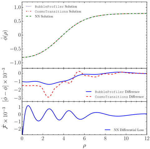
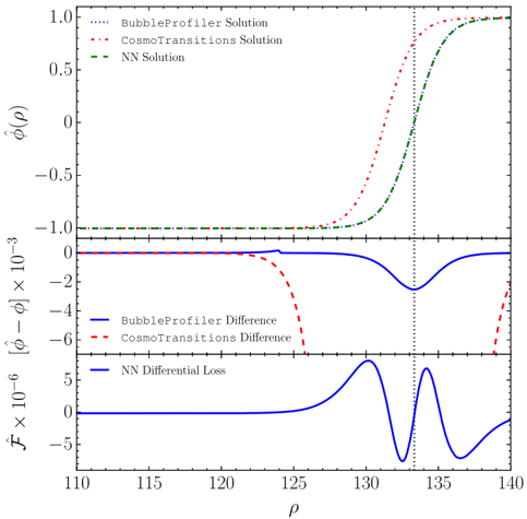
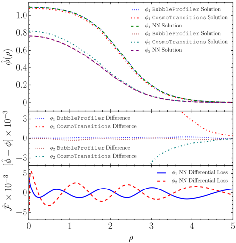
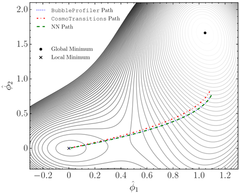
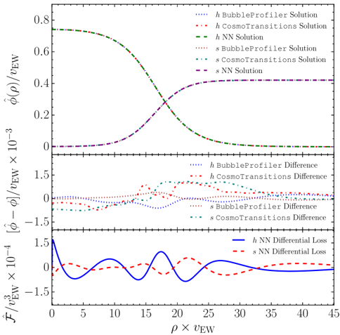
Starting from the observation that artificial neural networks are uniquely suited to solving optimization problems, and most physics problems can be cast as an optimization task, we introduce a novel way of finding a numerical solution to wide classes of differential equations. We find our approach to be very flexible and stable without relying on trial solutions, and applicable to ordinary, partial and coupled differential equations. We apply our method to the calculation of tunneling profiles for cosmological phase transitions, which is a problem of relevance for baryogenesis and stochastic gravitational wave spectra. Comparing our solutions with publicly available codes which use numerical methods optimized for the calculation of tunneling profiles, we find our approach to provide at least as accurate results as these dedicated differential equation solvers, and for some parameter choices, even more accurate and reliable solutions. In particular, we compare the neural network approach with two publicly available profile solvers, CosmoTransitions and BubbleProfiler, and give explicit examples where the neural network approach finds the correct solution while dedicated solvers do not. We point out that this approach of using artificial neural networks to solve equations is viable for any problem that can be cast into the form $\mathcal{F}(\stackrel{\ensuremath{\rightarrow}}{x})=0$, and is thus applicable to various other problems in perturbative and nonperturbative quantum field theory.
Overview
The claims and statistics of this paper haven’t been checked yet.
Run the check — free, no account needed. It reads the open-access text and checks the sources it cites.
Integrity signals
Registry
Cites
Statistics
Figures
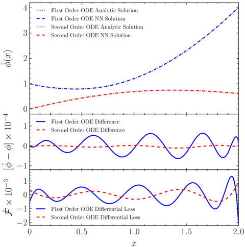
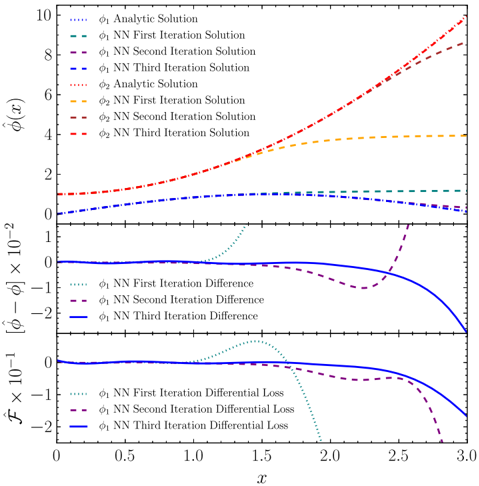
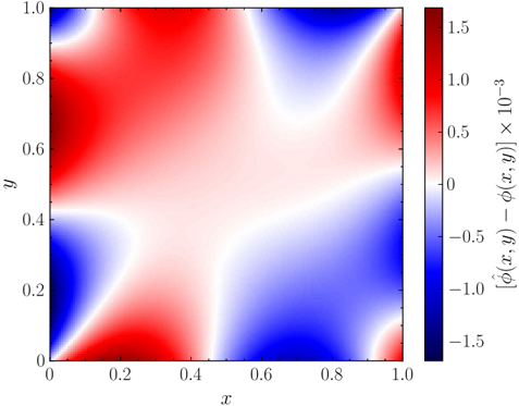
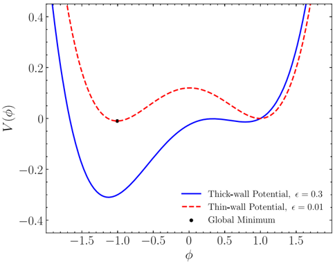
Verification
Claims the paper makes
The claims and statistics of this paper haven’t been checked yet.
Run the check — free, no account needed. It reads the open-access text and checks the sources it cites.
Claims other papers make about this one
Each is checked against this paper’s own text: does it say what the citing paper says it does?
In the citing paper
“Incorporating the current 2σ bound on the tensor/scalar ratio r [75, 76] requires roughly H/M P < 10 -7 .”
From Hyperbolic compactification of M-theory and de Sitter quantum gravity (2022) · cites this paper as [75]
Self-check
Percentages, sums and reported differences re-computed from the paper’s own numbers.
The self-check needs the paper’s full text.
Citations
Cites
Multilayer feedforward networks are universal approximators
Hornik, K., Stinchcombe, M., & White, H. (1989) · Neural Networks · doi:10.1016/0893-6080(89)90020-8 · Cited by 21,728
Approximation capabilities of multilayer feedforward networks
Hornik, K. (1991) · Neural Networks · doi:10.1016/0893-6080(91)90009-t · Cited by 6,091
On anomalous electroweak baryon-number non-conservation in the early universe
Kuzmin, V. A., Rubakov, V. A., & Shaposhnikov, M. E. (1985) · Physics Letters B · doi:10.1016/0370-2693(85)91028-7 · Cited by 3,008
Fate of the false vacuum: Semiclassical theory
Coleman, S. (1977) · Physical Review D · doi:10.1103/physrevd.15.2929 · Cited by 2,552
Violation of CP in variance, C asymmetry, and baryon asymmetry of the universe
Sakharov, A. D. (1991) · Soviet Physics Uspekhi · doi:10.1070/pu1991v034n05abeh002497 · Cited by 1,561
The Minimal Model of nonbaryonic dark matter: a singlet scalar
Burgess, C. P., Pospelov, M., & ter Veldhuis, T. (2001) · Nuclear Physics B · doi:10.1016/s0550-3213(01)00513-2 · Cited by 955
Caprini, C., Hindmarsh, M., Huber, S., Konstandin, T., Kozaczuk, J., Nardini, G., No, J. M., Petiteau, A., Schwaller, P., Servant, G., et al. (2016) · Journal of Cosmology and Astroparticle Physics · doi:10.1088/1475-7516/2016/04/001 · Cited by 927
Morrissey, D. E., & Ramsey-Musolf, M. J. (2012) · New Journal of Physics · doi:10.1088/1367-2630/14/12/125003 · Cited by 852
Decay of the false vacuum at finite temperature
Linde, A. D. (1983) · Nuclear Physics B · doi:10.1016/0550-3213(83)90293-6 · Cited by 829
The Minimal Model of Nonbaryonic Dark Matter: A Singlet ScalarPreprint
Burgess, C. P., Pospelov, M., & ter Veldhuis, T. (2000) · Cited by 601
Research works printed but not linked: 3
- M. E. Shaposhnikov, 1986, JETP Lett., 44, 465
- A. D. Linde, 1990, Contemp. Concepts Phys., 5, 1
- L. V. Kantorovich, 1948, Usp. Math. Nauk, 3, 89
Cited by
Hyperbolic compactification of M-theory and de Sitter quantum gravity
De Luca, G. B., Silverstein, E., & Torroba, G. (2022) · SciPost Physics · doi:10.21468/scipostphys.12.3.083 · Cited by 39
Metadata
- Authors
- Piscopo, M. L., Spannowsky, M., & Waite, P.
- ORCID
- Waite, Philip
- Venue
- Physical Review D
- Publisher
- American Physical Society (APS)
- Published
- 2019-07-09
- Volume
- 100
- Issue
- 1
- ISSN
- 2470-0010
- 2470-0029
- Cited by
- 117
- References
- 74
- Language
- en
- Funders
- University of Tuebingen
- Humboldt Society
About these checks
Registry, retraction, Cites and statistics results are computed, not judged, with one exception: a printed reference that no index lists is read once by a model before it counts as a citation error. Claims are extracted by a model and kept only when their quote appears verbatim in the text; each cited source is then checked, with a model’s help, for whether it says what the claim relies on. Those verdicts can be wrong — read the claim’s quote and the cited source before relying on one.
Statistics and arithmetic are recomputed, not judged.
Confidence bands are shown only for fields calibrated on our annotated test set. None is calibrated yet, so no band is shown.
What counts as a claim ›How we measure confidence ›How we check this ›
Are you an author, or do you see a problem with this page? Request a review
Data sources
Bibliographic data: Semantic Scholar, OpenAlex, Crossref.
Contains information from the Semantic Scholar Academic Graph Datasets, made available under the ODC Attribution License (ODC-BY 1.0).
Semantic Scholar’s data is described in: Kinney, R., et al. (2023). The Semantic Scholar Open Data Platform. arXiv:2301.10140.
