

The DOI matches its Crossref record; 44 of the 44 references it cites were found in a registry or an index.
Methods for testing publication bias in ecological and evolutionary meta‐analyses
Abstract
Publication bias threatens the validity of quantitative evidence from meta‐analyses as it results in some findings being overrepresented in meta‐analytic datasets because they are published more frequently or sooner (e.g. ‘positive’ results). Unfortunately, methods to test for the presence of publication bias, or assess its impact on meta‐analytic results, are unsuitable for datasets with high heterogeneity and non‐independence, as is common in ecology and evolutionary biology. We first review both classic and emerging publication bias tests (e.g. funnel plots, Egger's regression, cumulative meta‐analysis, fail‐safe N , trim‐and‐fill tests, p ‐curve and selection models), showing that some tests cannot handle heterogeneity, and, more importantly, none of the methods can deal with non‐independence. For each method, we estimate current usage in ecology and evolutionary biology, based on a representative sample of 102 meta‐analyses published in the last 10 years. Then, we propose a new method using multilevel meta‐regression, which can model both heterogeneity and non‐independence, by extending existing regression‐based methods (i.e. Egger's regression). We describe how our multilevel meta‐regression can test not only publication bias, but also time‐lag bias, and how it can be supplemented by residual funnel plots. Overall, we provide ecologists and evolutionary biologists with practical recommendations on which methods are appropriate to employ given independent and non‐independent effect sizes. No method is ideal, and more simulation studies are required to understand how Type 1 and Type 2 error rates are impacted by complex data structures. Still, the limitations of these methods do not justify ignoring publication bias in ecological and evolutionary meta‐analyses.
Overview
The claims and statistics of this paper haven’t been checked yet.
Run the check — free, no account needed. It reads the open-access text and checks the sources it cites.
Integrity signals
Registry
Cites
Statistics
Figures
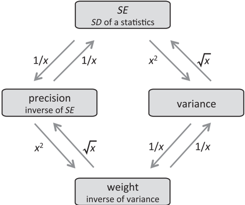
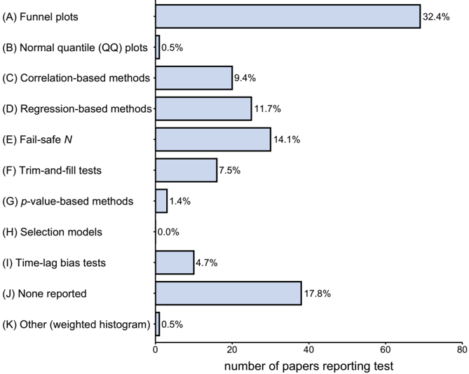
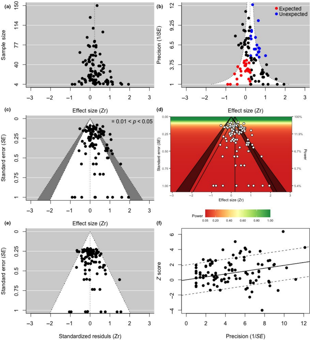
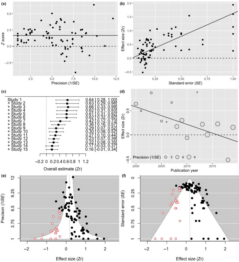
Verification
Claims the paper makes
The claims and statistics of this paper haven’t been checked yet.
Run the check — free, no account needed. It reads the open-access text and checks the sources it cites.
Claims other papers make about this one
Each is checked against this paper’s own text: does it say what the citing paper says it does?
In the citing paper
“Publication bias was visually assessed via funnel plots for multilevel meta-analysis using the code provided by Fernández-Castilla and colleagues243, and formally with the three-level version of Egger’s regression test244,245.”
From Prevalence and severity of mental health problems in early-career researchers: a systematic review and meta-analysis (2026) · cites this paper as [244]
Self-check
Percentages, sums and reported differences re-computed from the paper’s own numbers.
The self-check needs the paper’s full text.
Citations
Cites
Quantifying heterogeneity in a meta‐analysis
Higgins, J. P. T., & Thompson, S. G. (2002) · Statistics in Medicine · doi:10.1002/sim.1186 · Cited by 36,763
Conducting Meta-Analyses in R with the metafor Package
Viechtbauer, W. (2010) · Journal of Statistical Software · doi:10.18637/jss.v036.i03 · Cited by 20,464
Operating characteristics of a rank correlation test for publication bias
Begg, C. B., & Mazumdar, M. (1994) · Biometrics · doi:10.2307/2533446 · Cited by 16,955
Borenstein, M., Hedges, L. V., Higgins, J. P. T., & Rothstein, H. R. (2009) · doi:10.1002/9780470743386 · Cited by 14,225
Duval, S., & Tweedie, R. (2000) · Biometrics · doi:10.1111/j.0006-341x.2000.00455.x · Cited by 14,099
The file drawer problem and tolerance for null results.
Rosenthal, R. (1979) · Psychological Bulletin · doi:10.1037/0033-2909.86.3.638 · Cited by 9,068 · cited 3×
“Fail-safe N (also known as the ‘file-drawer number’) represents the number of non-302 significant unpublished results needed to exist to make the overall effect non-significant (e.g., Rosenthal, 1979; Rosenberg, 2005) or negligible in magnitude (e.g., Owrin, 1983).”
InfluentialSterne, J. A. C., Sutton, A. J., Ioannidis, J. P. A., Terrin, N., Jones, D. R., Lau, J., Carpenter, J., Rucker, G., Harbord, R. M., Schmid, C. H., et al. (2011) · BMJ · doi:10.1136/bmj.d4002 · Cited by 7,709
Simmons, J. P., Nelson, L. D., & Simonsohn, U. (2011) · Psychological Science · doi:10.1177/0956797611417632 · Cited by 6,567
The meta-analysis of response ratios in experimental ecology
Hedges, L. V., Gurevitch, J., & Curtis, P. S. (1999) · Ecology · doi:10.1890/0012-9658(1999)080[1150:tmaorr]2.0.co;2 · Cited by 4,704
The Handbook of Research Synthesis and Meta-Analysis
(2019) · doi:10.7758/9781610448864 · Cited by 4,553
A Nonparametric “Trim and Fill” Method of Accounting for Publication Bias in Meta-Analysis
Duval, S., & Tweedie, R. (2000) · Journal of the American Statistical Association · doi:10.1080/01621459.2000.10473905 · Cited by 2,955
Publication Bias in Meta‐Analysis: Prevention, Assessment and Adjustments
(2005) · doi:10.1002/0470870168 · Cited by 2,368
Investigating and dealing with publication and other biases in meta-analysis
Sterne, J. A. C., Egger, M., & Smith, G. D. (2001) · BMJ · doi:10.1136/bmj.323.7304.101 · Cited by 2,225
A Fail-Safe N for Effect Size in Meta-Analysis
Orwin, R. G. (1983) · Journal of Educational Statistics · doi:10.2307/1164923 · Cited by 2,064 · cited 1×
“Fail-safe N (also known as the ‘file-drawer number’) represents the number of non-302 significant unpublished results needed to exist to make the overall effect non-significant (e.g., Rosenthal, 1979; Rosenberg, 2005) or negligible in magnitude (e.g., Owrin, 1983).”
Peters, J. L., Sutton, A. J., Jones, D. R., Abrams, K. R., & Rushton, L. (2008) · Journal of Clinical Epidemiology · doi:10.1016/j.jclinepi.2007.11.010 · Cited by 2,053
Doing Meta-Analysis with R: A Hands-On Guide
Harrer, M., Cuijpers, P., Furukawa, T. A., & Ebert, D. D. (2021) · doi:10.1201/9781003107347 · Cited by 1,850
Meta-analysis and the science of research synthesis
Gurevitch, J., Koricheva, J., Nakagawa, S., & Stewart, G. (2018) · Nature · doi:10.1038/nature25753 · Cited by 1,709
Self-citationP-curve: A key to the file-drawer.
Simonsohn, U., Nelson, L. D., & Simmons, J. P. (2014) · Journal of Experimental Psychology: General · doi:10.1037/a0033242 · Cited by 1,500
A comparison of methods to detect publication bias in meta‐analysis
Macaskill, P., Walter, S. D., & Irwig, L. (2001) · Statistics in Medicine · doi:10.1002/sim.698 · Cited by 1,286
Rosenberg, M. S. (2005) · Evolution · doi:10.1111/j.0014-3820.2005.tb01004.x · Cited by 1,285 · cited 3×
“Fail-safe N (also known as the ‘file-drawer number’) represents the number of non-302 significant unpublished results needed to exist to make the overall effect non-significant (e.g., Rosenthal, 1979; Rosenberg, 2005) or negligible in magnitude (e.g., Owrin, 1983).”
InfluentialSchwarzer, G., Carpenter, J. R., & Rücker, G. (2015) · Use R! · doi:10.1007/978-3-319-21416-0 · Cited by 1,230
Methodological issues and advances in biological meta-analysis
Nakagawa, S., & Santos, E. S. A. (2012) · Evolutionary Ecology · doi:10.1007/s10682-012-9555-5 · Cited by 1,032
Self-citationStanley, T. D., & Doucouliagos, H. (2014) · Research Synthesis Methods · doi:10.1002/jrsm.1095 · Cited by 916
Shi, L., & Lin, L. (2019) · Medicine · doi:10.1097/md.0000000000015987 · Cited by 818
Peters, J. L., Sutton, A. J., Jones, D. R., Abrams, K. R., & Rushton, L. (2007) · Statistics in Medicine · doi:10.1002/sim.2889 · Cited by 716
Correcting for Bias in Psychology: A Comparison of Meta-Analytic Methods
Carter, E. C., Schönbrodt, F. D., Gervais, W. M., & Hilgard, J. (2019) · Advances in Methods and Practices in Psychological Science · doi:10.1177/2515245919847196 · Cited by 588
Meta-evaluation of meta-analysis: ten appraisal questions for biologists
Nakagawa, S., Noble, D. W. A., Senior, A. M., & Lagisz, M. (2017) · BMC Biology · doi:10.1186/s12915-017-0357-7 · Cited by 579
Self-citationDuval, S. (2005) · Publication Bias in Meta‐Analysis · doi:10.1002/0470870168.ch8 · Cited by 496
Rodgers, M. A., & Pustejovsky, J. E. (2021) · Psychological Methods · doi:10.1037/met0000300 · Cited by 492
McShane, B. B., Böckenholt, U., & Hansen, K. T. (2016) · Perspectives on Psychological Science · doi:10.1177/1745691616662243 · Cited by 398
Moreno, S. G., Sutton, A. J., Ades, A., Stanley, T. D., Abrams, K. R., Peters, J. L., & Cooper, N. J. (2009) · BMC Medical Research Methodology · doi:10.1186/1471-2288-9-2 · Cited by 373
Testing for funnel plot asymmetry of standardized mean differences
Pustejovsky, J. E., & Rodgers, M. A. (2019) · Research Synthesis Methods · doi:10.1002/jrsm.1332 · Cited by 354
Sterne, J. A. C., Becker, B. J., & Egger, M. (2005) · Publication Bias in Meta‐Analysis · doi:10.1002/0470870168.ch5 · Cited by 341
Heterogeneity in ecological and evolutionary meta‐analyses: its magnitude and implications
Senior, A. M., Grueber, C. E., Kamiya, T., Lagisz, M., O'Dwyer, K., Santos, E. S. A., & Nakagawa, S. (2016) · Ecology · doi:10.1002/ecy.1591 · Cited by 299
Self-citationComparing meta-analyses and preregistered multiple-laboratory replication projects
Kvarven, A., Strømland, E., & Johannesson, M. (2019) · Nature Human Behaviour · doi:10.1038/s41562-019-0787-z · Cited by 271
Meta-analysis using effect size distributions of only statistically significant studies.
van Assen, M. A. L. M., van Aert, R. C. M., & Wicherts, J. M. (2015) · Psychological Methods · doi:10.1037/met0000025 · Cited by 265
Hedges, L. V. (1984) · Journal of Educational Statistics · doi:10.3102/10769986009001061 · Cited by 241
Limitations of PET-PEESE and Other Meta-Analysis Methods
Stanley, T. D. (2017) · Social Psychological and Personality Science · doi:10.1177/1948550617693062 · Cited by 229
van Aert, R. C. M., Wicherts, J. M., & van Assen, M. A. L. M. (2016) · Perspectives on Psychological Science · doi:10.1177/1745691616650874 · Cited by 219
A historical review of publication bias
Marks‐Anglin, A., & Chen, Y. (2020) · Research Synthesis Methods · doi:10.1002/jrsm.1452 · Cited by 165
Havranek, T., & Sokolova, A. (2020) · Review of Economic Dynamics · doi:10.1016/j.red.2019.05.004 · Cited by 141
Finding the power to reduce publication bias
Stanley, T. D., Doucouliagos, H., & Ioannidis, J. P. A. (2017) · Statistics in Medicine · doi:10.1002/sim.7228 · Cited by 131
VEVEA, J. L., COBURN, K., & SUTTON, A. (2019) · The Handbook of Research Synthesis and Meta-Analysis · doi:10.7758/9781610448864.21 · Cited by 96
An assessment of statistical methods for nonindependent data in ecological meta‐analyses
Song, C., Peacor, S. D., Osenberg, C. W., & Bence, J. R. (2020) · Ecology · doi:10.1002/ecy.3184 · Cited by 71 · cited 1×
“Overall means will generally not be biased using aggregated or single sample/study effect sizes (Song et al. , 2020).”
Research works printed but not linked: 58
- 10.1002/sim.8422 · DOI
- 10.1186/s12874‐020‐01137‐1 · DOI
- 10.1002/jrsm.1404 · DOI
- 10.1111/j.1600‐0706.2011.19401.x · DOI
- 10.1002/0470870168.ch7 · DOI
- 10.1002/jrsm.1441 · DOI
- 10.1037/met0000119 · DOI
- Cohen J., 1988, Statistical power analysis for the beahvioral sciences
- 10.1016/j.healthpol.2012.10.015 · DOI
- 10.1016/j.jclinepi.2005.01.016 · DOI · Paper page
- 10.1002/jrsm.1414 · DOI
- 10.1111/2041‐210X.12927 · DOI
- 10.1111/j.1467‐8543.2009.00723.x · DOI · Paper page
- 10.1136/bmj.315.7109.629 · DOI · Paper page
- 10.1080/00220973.2019.1582470 · DOI
- 10.1046/j.1365‐2656.2002.00618.x · DOI
- 10.1186/1471‐2288‐8‐32 · DOI
- 10.1002/sim.4780070807 · DOI
- 10.1111/2041‐210X.12758 · DOI
- 10.1111/j.1420‐9101.2009.01915.x · DOI
- 10.1016/j.jinteco.2011.07.004 · DOI
- Hedges L., 1985, Statistical methods for meta‐analysis
- 10.1002/jrsm.5 · DOI · Paper page
- 10.1007/s11121‐021‐01279‐8 · DOI
- 10.2307/3558999 · DOI
- 10.23943/princeton/9780691137285.003.0014 · DOI
- 10.1098/rspb.2001.1832 · DOI
- 10.1111/1365‐2745.12224 · DOI · Paper page
- 10.1515/9781400846184-017 · DOI
- 10.1016/j.tree.2019.05.006 · DOI
- 10.1027/2151‐2604/a000392 · DOI
- 10.1890/14‐2402.1 · DOI · Paper page
- 10.4159/9780674040243 · DOI
- 10.4310/SII.2020.v13.n4.a5 · DOI
- Marks‐Anglin A., 2021, Handbook of meta‐analysis, 283
- 10.1007/s10683‐021‐09716‐9 · DOI
- 10.1016/S0169‐5347(01)02235‐2 · DOI
- 10.1111/jeb.12945 · DOI
- 10.1002/ecy.3490 · DOI
- 10.1111/mec.14031 · DOI
- 10.1002/bimj.200610341 · DOI
- 10.1001/jama.295.6.676 · DOI · Paper page
- 10.1111/j.1365‐2753.2003.00457.x · DOI
- Roberts C. J., 2005, Meta‐regression analysis: Issues of publicaiton bias in economics
- 10.1002/sim.2971 · DOI
- 10.7554/eLife.37385 · DOI
- 10.1002/jrsm.1423 · DOI
- 10.1111/j.0950‐0804.2005.00250.x · DOI
- 10.4324/9780203111710 · DOI
- 10.2307/146404 · DOI
- 10.1016/j.jclinepi.2005.01.006 · DOI
- 10.1002/(SICI)1097‐0258(19991030)18:20<2693:AID‐SIM235>3.0.CO;2‐V · DOI
- 10.1002/0470870168.ch13 · DOI
- vanAert R. C. M. &vanAssen M. A. L. M.(2021).Correcting for publication bias in a meta‐analysis with the p‐uniform* Method.OSF preprint https://osf.io/ebq6m/
- 10.1007/BF02294384 · DOI
- 10.1002/jrsm.1042 · DOI
- 10.1007/978-0-387-98141-3 · DOI · Paper page
- 10.7554/eLife.24260 · DOI
Cited by
Sorted by citations
The biodiversity and ecosystem service contributions and trade-offs of forest restoration approaches
Hua, F., Bruijnzeel, L. A., Meli, P., Martin, P. A., Zhang, J., Nakagawa, S., Miao, X., Wang, W., McEvoy, C., Peña-Arancibia, J. L., et al. (2022) · Science · doi:10.1126/science.abl4649 · Cited by 831
Self-citationDownie, A. T., Wu, N. C., Cramp, R. L., & Franklin, C. E. (2023) · Global Change Biology · doi:10.1111/gcb.16848 · Cited by 34
Spindle-dependent memory consolidation in healthy adults: a meta-analysis
Kumral, D., Matzerath, A., Leonhart, R., & Schönauer, M. (2023) · Neuropsychologia · doi:10.1016/j.neuropsychologia.2023.108661 · Cited by 32
Thurston, C., Murray, A. L., Franchino-Olsen, H., Silima, M., Hemady, C. L., & Meinck, F. (2026) · Trauma, Violence, & Abuse · doi:10.1177/15248380251358223 · Cited by 25
“…test have been suggested (Egger et al., 1997; Fernández-Castilla et al., 2021; Stanley & Doucouliagos, 2014), including the addition of moderators such as a measure of precision of the estimates into the multilevel meta-analytic models to better account for heterogeneity (Nakagawa et al., 2022).”
Cait, J., Winder, C. B., & Mason, G. J. (2024) · Applied Animal Behaviour Science · doi:10.1016/j.applanim.2024.106361 · Cited by 21
Metadata
- Authors
- Nakagawa, S., Lagisz, M., Jennions, M. D., Koricheva, J., Noble, D. W. A., Parker, T. H., Sánchez‐Tójar, A., Yang, Y., & O'Dea, R. E.
- Venue
- Methods in Ecology and Evolution
- Publisher
- Wiley
- Published
- 2021-11-10
- Volume
- 13
- Issue
- 1
- Pages
- 4-21
- ISSN
- 2041-210X
- Cited by
- 399
- References
- 44
- Language
- en
- Update notices
- correction (2022-06-20)
- Funders
- Australian Research Council (DP200100367)
- Deutsche Forschungsgemeinschaft (316099922, 396782608)
About these checks
Registry, retraction, Cites and statistics results are computed, not judged, with one exception: a printed reference that no index lists is read once by a model before it counts as a citation error. Claims are extracted by a model and kept only when their quote appears verbatim in the text; each cited source is then checked, with a model’s help, for whether it says what the claim relies on. Those verdicts can be wrong — read the claim’s quote and the cited source before relying on one.
Statistics and arithmetic are recomputed, not judged.
Confidence bands are shown only for fields calibrated on our annotated test set. None is calibrated yet, so no band is shown.
What counts as a claim ›How we measure confidence ›How we check this ›
Are you an author, or do you see a problem with this page? Request a review
