

The DOI matches its Crossref record; 78 of the 78 references it cites were found in a registry or an index.
Comparison of co-expression measures: mutual information, correlation, and model based indices
Open accessAbstract
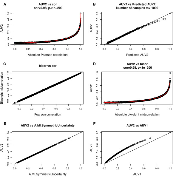
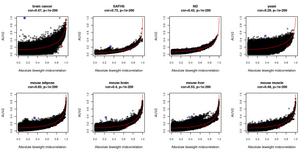
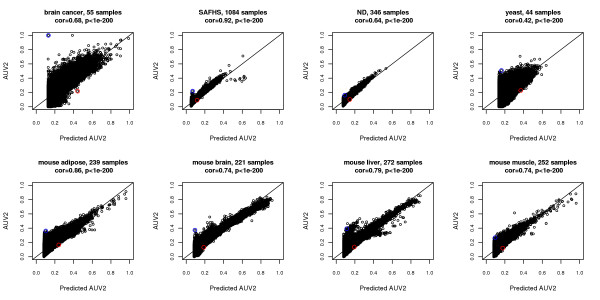
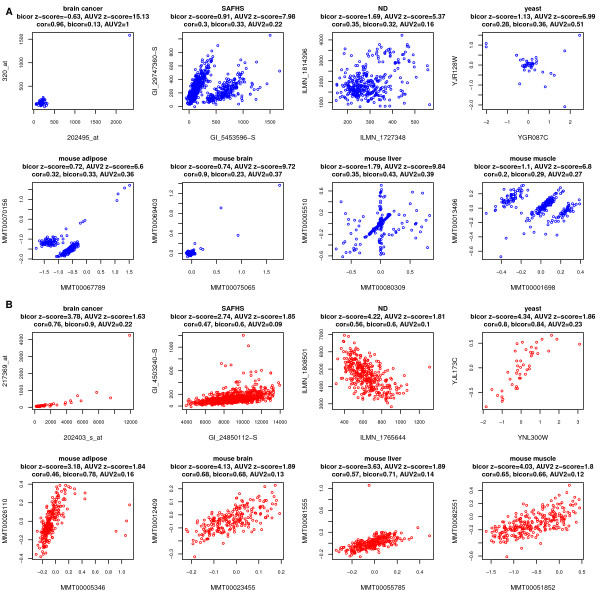
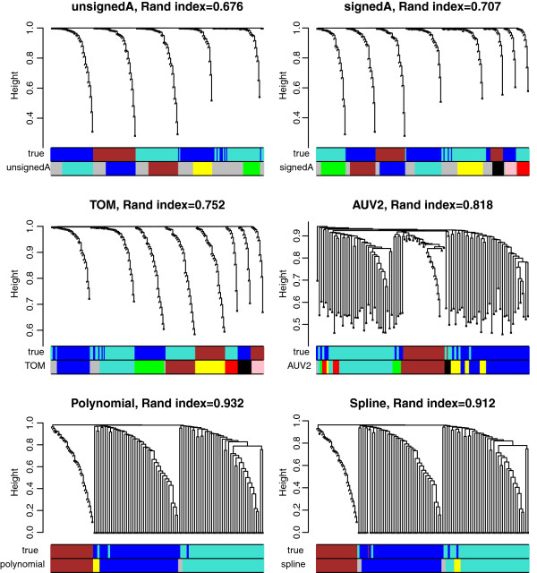
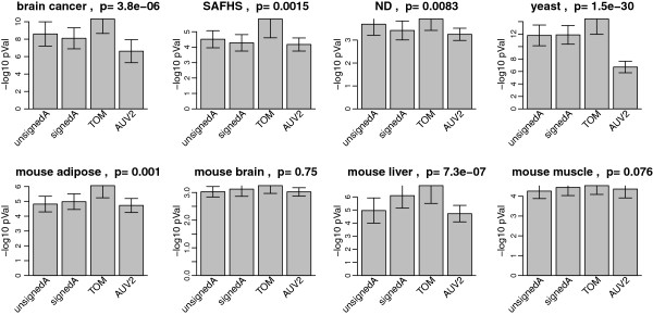
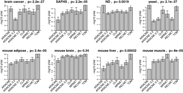
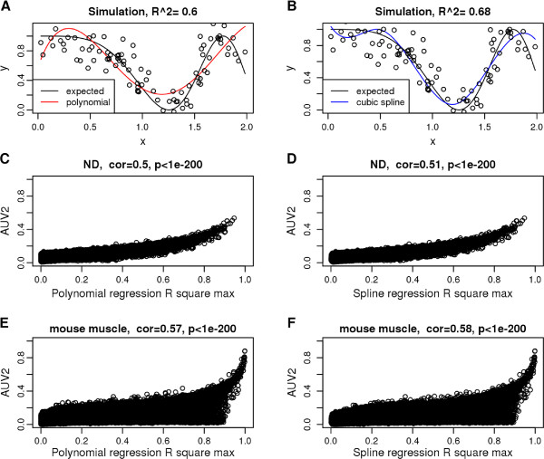
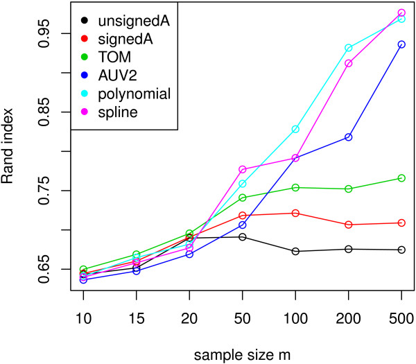
Background: Co-expression measures are often used to define networks among genes. Mutual information (MI) is often used as a generalized correlation measure. It is not clear how much MI adds beyond standard (robust) correlation measures or regression model based association measures. Further, it is important to assess what transformations of these and other co-expression measures lead to biologically meaningful modules (clusters of genes). Results: We provide a comprehensive comparison between mutual information and several correlation measures in 8 empirical data sets and in simulations. We also study different approaches for transforming an adjacency matrix, e.g. using the topological overlap measure. Overall, we confirm close relationships between MI and correlation in all data sets which reflects the fact that most gene pairs satisfy linear or monotonic relationships. We discuss rare situations when the two measures disagree. We also compare correlation and MI based approaches when it comes to defining co-expression network modules. We show that a robust measure of correlation (the biweight midcorrelation transformed via the topological overlap transformation) leads to modules that are superior to MI based modules and maximal information coefficient (MIC) based modules in terms of gene ontology enrichment. We present a function that relates correlation to mutual information which can be used to approximate the mutual information from the corresponding correlation coefficient. We propose the use of polynomial or spline regression models as an alternative to MI for capturing non-linear relationships between quantitative variables. Conclusion: The biweight midcorrelation outperforms MI in terms of elucidating gene pairwise relationships. Coupled with the topological overlap matrix transformation, it often leads to more significantly enriched co-expression modules. Spline and polynomial networks form attractive alternatives to MI in case of non-linear relationships. Our results indicate that MI networks can safely be replaced by correlation networks when it comes to measuring co-expression relationships in stationary data.
Overview
The claims and statistics of this paper haven’t been checked yet.
Run the check — free, no account needed. It reads the open-access text and checks the sources it cites.
Integrity signals
Registry
Cites
Statistics
Figures
Verification
Claims the paper makes
The claims and statistics of this paper haven’t been checked yet.
Run the check — free, no account needed. It reads the open-access text and checks the sources it cites.
Claims other papers make about this one
Each is checked against this paper’s own text: does it say what the citing paper says it does?
The source backs part of the claim, not all of it — or backs it for a different population, condition or comparison.
In the citing paper
“However, WGCNA's reliance on linear correlations and scale-free assumptions has drawn criticism for oversimplifying the nonlinear and heterogeneous nature of molecular interactions300.”
From Artificial intelligence-driven multi-omics approaches in Alzheimer's disease: Progress, challenges, and future directions (2025) · cites this paper as [300]
Experimental — accuracy not yet measuredThe check wasn’t confident either way, so it gives no verdict — never disputed.
In the citing paper
“At currently available sample sizes, networks are most reproducible at a module level35,38,39, then at the hub gene level41,223 and, last, at the level of precise gene connectivity rankings or precise module memberships of genes40,49.”
From Systems biology and gene networks in neurodevelopmental and neurodegenerative disorders (2015) · cites this paper as [38]
Experimental — accuracy not yet measuredIn the citing paper
“weighted networks constructed with the topological overlap of correlation (for example, by weighted gene co-expression network analysis (WGCNA)42,44) have similar sensitivity and specificity for detecting true network structure for experiments involving monotonic relationships as do networks constructed with nonlinear association measures such as mutual information (for example, by the Algorithm”
From Systems biology and gene networks in neurodevelopmental and neurodegenerative disorders (2015) · cites this paper as [38]
In the citing paper
“signed networks are more predictive of protein interactions and shared pathway relationships than unsigned networks38,42,43”
From Systems biology and gene networks in neurodevelopmental and neurodegenerative disorders (2015) · cites this paper as [38]
In the citing paper
“Interestingly, there was no pathway or PPI enrichment in these modules, probably owing to the inclusion of both positive and negative correlations when computing co-expression relationships (unsigned networks), which is a method that is less sensitive to pathway and protein interaction detection38,43.”
From Systems biology and gene networks in neurodevelopmental and neurodegenerative disorders (2015) · cites this paper as [38]
Self-check
Percentages, sums and reported differences re-computed from the paper’s own numbers.
The self-check needs the paper’s full text.
Citations
Cites
Gene Ontology: tool for the unification of biology
Ashburner, M., Ball, C. A., Blake, J. A., Botstein, D., Butler, H., Cherry, J. M., Davis, A. P., Dolinski, K., Dwight, S. S., Eppig, J. T., et al. (2000) · Nature Genetics · doi:10.1038/75556 · Cited by 43,206
Elements of Information Theory
Cover, T. M., & Thomas, J. A. (2001) · Wiley eBooks · doi:10.1002/0471200611 · Cited by 37,139
WGCNA: an R package for weighted correlation network analysis
Langfelder, P., & Horvath, S. (2008) · BMC Bioinformatics · doi:10.1186/1471-2105-9-559 · Cited by 27,252
Self-citationCluster analysis and display of genome-wide expression patterns
Eisen, M. B., Spellman, P. T., Brown, P. O., & Botstein, D. (1998) · Proceedings of the National Academy of Sciences · doi:10.1073/pnas.95.25.14863 · Cited by 16,184
Bioconductor: open software development for computational biology and bioinformatics
Gentleman, R. C., Carey, V. J., Bates, D. M., Bolstad, B., Dettling, M., Dudoit, S., Ellis, B., Gautier, L., Ge, Y., Gentry, J., et al. (2004) · Genome biology · doi:10.1186/gb-2004-5-10-r80 · Cited by 12,082
A General Framework for Weighted Gene Co-Expression Network Analysis
Zhang, B., & Horvath, S. (2005) · Statistical Applications in Genetics and Molecular Biology · doi:10.2202/1544-6115.1128 · Cited by 5,684
Self-citationMetabolic stability and epigenesis in randomly constructed genetic nets
Kauffman, S. A. (1969) · Journal of Theoretical Biology · doi:10.1016/0022-5193(69)90015-0 · Cited by 4,871
Spellman, P. T., Sherlock, G. J., Zhang, M. Q., Iyer, V. R., Anders, K. R., Eisen, M. B., Brown, P. O., Botstein, D., & Futcher, B. (1998) · Molecular Biology of the Cell · doi:10.1091/mbc.9.12.3273 · Cited by 4,724
Hierarchical Organization of Modularity in Metabolic Networks
Ravasz, E., Somera, A. L., Mongru, D. A., Oltvai, Z. N., & Barabási, A.-L. (2002) · Science · doi:10.1126/science.1073374 · Cited by 4,224
Detecting Novel Associations in Large Data Sets
Reshef, D. N., Reshef, Y., Finucane, H. K., Grossman, S. R., McVean, G., Turnbaugh, P. J., Lander, E. S., Mitzenmacher, M., & Sabeti, P. C. (2011) · Science · doi:10.1126/science.1205438 · Cited by 3,345
Cited by
Sorted by citations
Items 401–476 of 476
Network Medicine in the age of biomedical big dataPreprint
Sonawane, A. R., Weiss, S. T., Glass, K., & Sharma, A. (2019) · arXiv (Cornell University) · doi:10.48550/arxiv.1903.05449
Discovering Gene Co-Expression Modules Using Fuzzified Adjusted Rand Index
Adigun, T. O., & Makolo, A. U. (2019) · Computational Biology and Bioinformatics · doi:10.11648/j.cbb.20190702.11
Integration and visualisation of clinical-omics datasets for medical knowledge discovery
Homola, D. (2017) · Spiral (Imperial College London) · doi:10.25560/67647
Roberts, W. R., & Roalson, E. H. (2019) · bioRxiv (Cold Spring Harbor Laboratory) · doi:10.1101/817221
Bassignana, G., Fransson, J., Henry, V., Colliot, O., Zujovic, V., & Fallani, F. D. V. (2020) · arXiv (Cornell University) · doi:10.48550/arxiv.2003.08913
Transparent Machine Learning for Multi-Omics Analysis of Mental Disorders
Belin, S. (2020) · Uppsala University Publications (Uppsala University)
Data-Driven Statistical Approaches for Omics Data Analysis
Lü, J., & Wang, P. (2020) · Springer eBooks · doi:10.1007/978-981-15-9144-0_9
Structure Learning for Hierarchical Regulatory NetworksPreprint
Federico, A. N., Kern, J. G., Varelas, X., & Monti, S. (2021) · bioRxiv (Cold Spring Harbor Laboratory) · doi:10.1101/2021.05.27.446022
On Study of Mutual Information and its Estimation MethodsPreprint
Sinaga, M. A. (2021) · arXiv (Cornell University) · doi:10.48550/arxiv.2106.14646
Constructing Functional Networks of Phosphorylation Sites Using Co-PhosphorylationPreprint
Ayati, M., Yılmaz, S., Chance, M. R., & Koyutürk, M. (2021) · bioRxiv (Cold Spring Harbor Laboratory) · doi:10.1101/2021.08.16.456448
A Comparison Between Robust Methods in Canonical Correlation by Using Empirical Influence Function
Al-Ameed, Z. K., & Al-Always, L. A. (2021) · Journal of Economics and Administrative Sciences · doi:10.33095/jeas.v27i128.2163
AGEAS: Automated Machine Learning based Genetic Regulatory Element Extraction SystemPreprint
Nakamoto, M., Tao, J., & Yu, J. C.-K. (2022) · bioRxiv (Cold Spring Harbor Laboratory) · doi:10.1101/2022.02.17.480852
SGCP: a spectral self-learning method for clustering genes in co-expression networks
Aghaieabiane, N., & Koutis, I. (2024) · BMC Bioinformatics · doi:10.1186/s12859-024-05848-w · Cited by 2
Singh, P., Guo, J., Li, J., Singh, U., Wurtele, E. S., & Bassler, K. E. (2022) · bioRxiv (Cold Spring Harbor Laboratory) · doi:10.1101/2022.12.28.522153
A Network-based Approach for Inferring Thresholds in Co-expression Networks
López-Rozo, N., Romero, M., Finke, J., & Rocha, C. (2023) · Studies in computational intelligence · doi:10.1007/978-3-031-21127-0_22
li, Z., Song, C., Yang, J., Jia, Z., Yan, C., Tian, L., & Wu, X. (2023) · Research Square · doi:10.21203/rs.3.rs-2641728/v1
Graph Neural Networks to Identify Genetic Modifiers of Rare Complex Inheritable Diseases
Niktab, E. (2023) · Open Access Victoria University of Wellington | Te Herenga Waka (Figshare) · doi:10.26686/wgtn.22714963
Miao, X., & Zhang, S. (2023) · Frontiers in Science and Engineering · doi:10.54691/fse.v3i5.5005
Yue, Z., Yan, D., Guo, G., & Chen, J. Y. (2023) · Biostatistics Research · doi:10.37256/bsr.1120231921
A Novel Information Entropy Approach for Crack Monitoring Leveraging Nondestructive EvaluationPreprint
Malik, S., & Kontsos, A. (2023) · SSRN Electronic Journal · doi:10.2139/ssrn.4532349
ทรานสครปโทมของขาวพนธพนเมองไทยภายใตภาวะเครยดจากความเคม
จันทนกูล, พ., ชัชวาลย์, ศ., & พลายมาศ, ก. (2019) · doi:10.58837/chula.the.2019.1024
Network Development and Comparison in Lipidomics and Metabolomics
Nguyen-Tran, T., Alkassir, Q., Bennett, S. A. L., & Čuperlović‐Culf, M. (2023) · Springer eBooks · doi:10.1007/978-3-031-39094-4_2
Constructing a graphical representation of the brain from functional MRI
Bica, M. T. (2023) · Journal of Brain Sciences · doi:10.18488/83.v6i1.3582
Wei, R., Zhong, Y., Xu, N., Li, P., Azhar, M. T., Yang, Z., Zhao, Y., Yán, H., Liú, À., Gǒng, W., et al. (2024) · Industrial Crops and Products · doi:10.1016/j.indcrop.2024.118130
From local to global gene co-expression estimation using single-cell RNA-seq data
Tian, J., Lei, J., & Roeder, K. (2024) · Biometrics · doi:10.1093/biomtc/ujae001
Zhang, X., Li, J., Pan, B.-Z., Chen, W., Chen, M., Tang, M., Xu, Z., & Liu, C. (2021) · Figshare · doi:10.6084/m9.figshare.15253726
Zhang, X., Li, J., Pan, B.-Z., Chen, W., Chen, M., Tang, M., Xu, Z., & Liu, C. (2021) · Figshare · doi:10.6084/m9.figshare.15253735
Zhang, X., Li, J., Pan, B.-Z., Chen, W., Chen, M., Tang, M., Xu, Z., & Liu, C. (2021) · Figshare · doi:10.6084/m9.figshare.15253729
Zhang, X., Li, J., Pan, B.-Z., Chen, W., Chen, M., Tang, M., Xu, Z., & Liu, C. (2021) · Figshare · doi:10.6084/m9.figshare.15253771
Liu, Y., Ye, X., Yu, C. Y., Shao, W., Hou, J., Feng, W., Zhang, J., & Huang, K. (2021) · Figshare · doi:10.6084/m9.figshare.16864760
Zhang, Y., Shi, W., & Sun, Y. (2023) · Figshare · doi:10.6084/m9.figshare.22603484
Zhang, X., Li, J., Pan, B.-Z., Chen, W., Chen, M., Tang, M., Xu, Z., & Liu, C. (2021) · Figshare · doi:10.6084/m9.figshare.15253756
Zhang, X., Li, J., Pan, B.-Z., Chen, W., Chen, M., Tang, M., Xu, Z., & Liu, C. (2021) · Figshare · doi:10.6084/m9.figshare.15253711 · Cited by 1
Zhang, Y., Shi, W., & Sun, Y. (2023) · Figshare · doi:10.6084/m9.figshare.22603481
Zhang, X., Li, J., Pan, B.-Z., Chen, W., Chen, M., Tang, M., Xu, Z., & Liu, C. (2021) · Figshare · doi:10.6084/m9.figshare.15253723
Zhang, X., Li, J., Pan, B.-Z., Chen, W., Chen, M., Tang, M., Xu, Z., & Liu, C. (2021) · Figshare · doi:10.6084/m9.figshare.15253705
Zhang, X., Li, J., Pan, B.-Z., Chen, W., Chen, M., Tang, M., Xu, Z., & Liu, C. (2021) · Figshare · doi:10.6084/m9.figshare.15253747
Zhang, X., Li, J., Pan, B.-Z., Chen, W., Chen, M., Tang, M., Xu, Z., & Liu, C. (2021) · Figshare · doi:10.6084/m9.figshare.15253738
Zhang, X., Li, J., Pan, B.-Z., Chen, W., Chen, M., Tang, M., Xu, Z., & Liu, C. (2021) · Figshare · doi:10.6084/m9.figshare.15253714
Zhang, Y., Shi, W., & Sun, Y. (2023) · Figshare · doi:10.6084/m9.figshare.22603478
Zhang, X., Li, J., Pan, B.-Z., Chen, W., Chen, M., Tang, M., Xu, Z., & Liu, C. (2021) · Figshare · doi:10.6084/m9.figshare.15253774
Ghosh, S., Datta, R., & Thakur, S. (2024) · Human Gene · doi:10.1016/j.humgen.2024.201357
A Selective Review of Network Analysis Methods for Gene Expression Data
Li, R., Yi, H., & Ma, S. (2025) · Methods in molecular biology · doi:10.1007/978-1-0716-4276-4_14
Han, M., Chen, X., Li, X., Ma, J., Chen, T., Yang, C., Wang, J., Li, Y., Guo, W., & Zhu, Y. (2025) · Briefings in Bioinformatics · doi:10.1093/bib/bbaf081 · Cited by 1
Yousaf, M., Shafique, L., Qamar, S., Shakeel, M., Ali, F., & Ali, Z. (2025) · Environmental Monitoring and Assessment · doi:10.1007/s10661-025-14578-2
Principles, methods and applications of gene regulatory network inference
Jiang, Y., Liu, Z., Zhang, Q., Chen, Z., Zan, Z., Lü, Q., Wang, J., Zhu, J., Zhang, J., & Wei, X. (2025) · Scientia Sinica Vitae · doi:10.1360/ssv-2025-0070
Fu, X., Wang, J., Gu, C., & Zou, H. (2025) · Chinese Journal of Physics · doi:10.1016/j.cjph.2025.11.004
Abdullahi, M. S., Piro, R. M., Suratanee, A., & Plaimas, K. (2025) · Computational and Structural Biotechnology Journal · doi:10.1016/j.csbj.2025.11.018
tGeCoNet: a framework for constructing temporal gene co-expression networks
Cinaglia, P. (2025) · Neurocomputing · doi:10.1016/j.neucom.2025.132151
Huang, M., Modeste, E. S., Dammer, E., Merino, P., Taylor, G., Duong, D. M., Deng, Q., Holler, C. J., Gearing, M., Dickson, D. W., et al. (2020) · Figshare · doi:10.6084/m9.figshare.13064301
Lemoine, G. G., Scott‐Boyer, M., Ambroise, B., Périn, O., & Droit, A. (2021) · Figshare · doi:10.6084/m9.figshare.14677009
Huang, M., Modeste, E. S., Dammer, E., Merino, P., Taylor, G., Duong, D. M., Deng, Q., Holler, C. J., Gearing, M., Dickson, D. W., et al. (2020) · Figshare · doi:10.6084/m9.figshare.13064298
Zhang, X., Li, J., Pan, B.-Z., Chen, W., Chen, M., Tang, M. T., Xu, Z.-F., & Liu, C. (2021) · Figshare · doi:10.6084/m9.figshare.15253720
Additional file 2 of Cestode strobilation: prediction of developmental genes and pathways
Paludo, G. P., Thompson, C. E., Miyamoto, K. N., Guedes, R. L. M., Zaha, A., de Vasconcelos, A. T. R., Cancela, M., & Ferreira, H. B. (2020) · Figshare · doi:10.6084/m9.figshare.12667880
Chang, L.-Y., Hao, T.-Y., Wang, W.-J., & Lin, C.-Y. (2024) · Figshare · doi:10.6084/m9.figshare.26952273
Liu, Y., Ye, X., Yu, C. Y., Shao, W., Hou, J., Feng, W., Zhang, J., & Huang, K. (2021) · Figshare · doi:10.6084/m9.figshare.16864757
Network-Based Diseasome Construction From Multi-Omics Data and RadTrix Visualization
Bitra, V. S., Vangimalla, R. R., & Sreevalsan‐Nair, J. (2025) · IEEE Transactions on Computational Biology and Bioinformatics · doi:10.1109/tcbbio.2025.3599771
Changes in transposable elements expression in male and female mice liver throughout aging
Hernández, B., Murgas, P., & Riadi, G. (2026) · GeroScience · doi:10.1007/s11357-025-02065-y
Rabiei, P., Massé‐Alarie, H., & Desrosiers, P. (2026) · medRxiv · doi:10.64898/2026.02.09.26345929
Valdeolivas, A. (2019) · theses.fr (ABES) · doi:10.70675/5379aa9cz8f24z45c6z8d81z2e0796525163
Methodological developments for omic data integration : applications to oncology and neurosciences
Brière, G. (2022) · theses.fr (ABES) · doi:10.70675/13a03fd5zc563z49a8zb32az6cab055621d9
Bampos, C., & Megalooikonomou, V. (2026) · PLoS ONE · doi:10.1371/journal.pone.0346663
Rutao, X., Xiong, Z., Jichun, Z., Zheng, T., Kewei, Z., Qingqing, W., Ding, Y., Xiyang, C., Chengxin, W., & Bin, H. (2026) · Human Mutation · doi:10.1155/humu/7210691
A Rāga Independent Encoder for Svara Representation in Carnatic Music
Vijayan, V., Nuttall, T., & Serra, X. (2026) · International Conference on Digital Libraries for Musicology (DLfM) · doi:10.1145/3815723.3815730
Zhou, L., Luo, S., Huang, Z., Zhang, Z., Wang, Z., & Zhang, J. (2026) · Molecular Systems Biology · doi:10.1038/s44320-026-00235-4 · Cited by 1
Guaranteed Discovery of Control-Endogenous Latent States with Multi-Step Inverse Models
Lamb, A., Islam, R., Efroni, Y., Didolkar, A., Misra, D., Foster, D., Molu, L., Chari, R., Krishnamurthy, A., & Langford, J. (2022) · arXiv · doi:10.48550/arxiv.2207.08229 · Cited by 1
Metadata
- Authors
- Song, L., Langfelder, P., & Horvath, S.
- Affiliations
- University of California, Los Angeles (US)
- Corresponding author
- Horvath, Steve
- Venue
- BMC Bioinformatics
- Published
- 2012-12
- Volume
- 13
- Issue
- 1
- Pages
- 328-328
- ISSN
- 1471-2105 (ISSN-L)
- PMC
- PMC3586947
- OpenAlex
- W2133254377
- Cited by
- 460
- References
- 78
- Citations by year
- 2026: 9 · 2025: 27 · 2024: 34 · 2023: 35 · 2022: 48 · 2021: 49 · 2020: 51 · 2019: 47 · 2018: 36 · 2017: 33 · 2016: 38 · 2015: 25 · 2014: 18 · 2013: 8 · 2012: 2
- FWCI
- 6.82
- Type
- journal article
- Language
- en
- Open access
- gold
- doi.org
- Licence
- cc-by
- Locations
- BMC Bioinformatics (publishedVersion, cc-by)
- Europe PMC (PubMed Central) (publishedVersion, cc-by)
- PubMed Central (publishedVersion, cc-by)
- PubMed (publishedVersion)
- DOAJ (DOAJ: Directory of Open Access Journals) (submittedVersion)
- eScholarship (California Digital Library) (submittedVersion)
- Funders
- National Institute on Drug Abuse (R01DA030913)
- National Cancer Institute (P50CA092131)
- National Institute of Neurological Disorders and Stroke (R01NS058980)
- Clinical and Translational Science Institute, University of California, Los Angeles
- Topics
- Life Sciences › Biochemistry, Genetics and Molecular Biology › Molecular Biology › Bioinformatics and Genomic Networks
- Life Sciences › Biochemistry, Genetics and Molecular Biology › Molecular Biology › Gene expression and cancer classification
- Life Sciences › Biochemistry, Genetics and Molecular Biology › Molecular Biology › Gene Regulatory Network Analysis
- Keywords
- mutual information, gene co-expression network, correlation measures, gene modules, maximal information coefficient, spline regression, polynomial regression, gene ontology enrichment
- MeSH terms
- Algorithms, Multigene Family, Humans, Models, Genetic, Statistics as Topic, Gene Expression Profiling, Gene Regulatory Networks
About these checks
Registry, retraction, Cites and statistics results are computed, not judged, with one exception: a printed reference that no index lists is read once by a model before it counts as a citation error. Claims are extracted by a model and kept only when their quote appears verbatim in the text; each cited source is then checked, with a model’s help, for whether it says what the claim relies on. Those verdicts can be wrong — read the claim’s quote and the cited source before relying on one.
Statistics and arithmetic are recomputed, not judged.
Confidence bands are shown only for fields calibrated on our annotated test set. None is calibrated yet, so no band is shown.
What counts as a claim ›How we measure confidence ›How we check this ›
Are you an author, or do you see a problem with this page? Request a review
