

The DOI matches its Crossref record; 36 of the 36 references it cites were found in a registry or an index.
Empirical array quality weights in the analysis of microarray data
Open accessAbstract
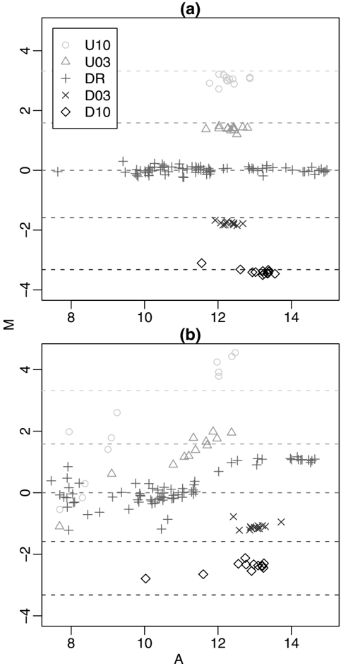
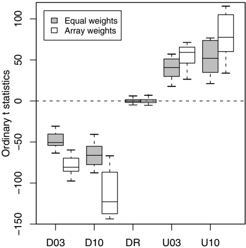
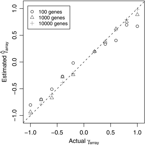
BACKGROUND: Assessment of array quality is an essential step in the analysis of data from microarray experiments. Once detected, less reliable arrays are typically excluded or "filtered" from further analysis to avoid misleading results. RESULTS: In this article, a graduated approach to array quality is considered based on empirical reproducibility of the gene expression measures from replicate arrays. Weights are assigned to each microarray by fitting a heteroscedastic linear model with shared array variance terms. A novel gene-by-gene update algorithm is used to efficiently estimate the array variances. The inverse variances are used as weights in the linear model analysis to identify differentially expressed genes. The method successfully assigns lower weights to less reproducible arrays from different experiments. Down-weighting the observations from suspect arrays increases the power to detect differential expression. In smaller experiments, this approach outperforms the usual method of filtering the data. The method is available in the limma software package which is implemented in the R software environment. CONCLUSION: This method complements existing normalisation and spot quality procedures, and allows poorer quality arrays, which would otherwise be discarded, to be included in an analysis. It is applicable to microarray data from experiments with some level of replication.
Overview
The claims and statistics of this paper haven’t been checked yet.
Run the check — free, no account needed. It reads the open-access text and checks the sources it cites.
Integrity signals
Registry
Cites
Statistics
Figures
Verification
Claims the paper makes
The claims and statistics of this paper haven’t been checked yet.
Run the check — free, no account needed. It reads the open-access text and checks the sources it cites.
Claims other papers make about this one
Each is checked against this paper’s own text: does it say what the citing paper says it does?
In the citing paper
“Probe and array weights can be easily combined by multiplying them together and, when used appropriately, have been demonstrated to increase power to detect DE (11,43).”
From limma powers differential expression analyses for RNA-sequencing and microarray studies (2015) · cites this paper as [11]
Self-check
Percentages, sums and reported differences re-computed from the paper’s own numbers.
The self-check needs the paper’s full text.
Citations
Cites
R: A Language and Environment for Statistical Computing
R Core Team (2000) · doi:10.32614/r.manuals · Cited by 355,893
Controlling the False Discovery Rate: A Practical and Powerful Approach to Multiple Testing
Benjamini, Y., & Hochberg, Y. (1995) · Journal of the Royal Statistical Society Series B: Statistical Methodology · doi:10.1111/j.2517-6161.1995.tb02031.x · Cited by 109,482
Smyth, G. K. (2004) · Statistical Applications in Genetics and Molecular Biology · doi:10.2202/1544-6115.1027 · Cited by 11,829
Self-citationlimma: Linear Models for Microarray Data
Smyth, G. K. (2005) · Statistics for Biology and Health · doi:10.1007/0-387-29362-0_23 · Cited by 5,796
Self-citationBioinformatics and Computational Biology Solutions Using R and Bioconductor
Gentleman, R. C., Carey, V. J., Huber, W. K., Irizarry, R. A., & Dudoit, S. (2005) · Statistics in the health sciences · doi:10.1007/0-387-29362-0 · Cited by 3,470
Normalization of cDNA microarray data
Smyth, G. K., & Speed, T. (2003) · Methods · doi:10.1016/s1046-2023(03)00155-5 · Cited by 1,871
Self-citationStatistical Analysis of Gene Expression Microarray Data
Speed, T. (2003) · Chapman & Hall/CRC eBooks · doi:10.1201/9780203011232 · Cited by 551
Statistical Issues in cDNA Microarray Data Analysis
Smyth, G. K., Yang, J. Y. H., & Speed, T. P. (2003) · Humana Press eBooks · doi:10.1385/1-59259-364-x:111 · Cited by 471
Self-citationComparison of Methods for Image Analysis on cDNA Microarray Data
Yang, J. Y. H., Buckley, M. J., Dudoit, S., & Speed, T. P. (2002) · Journal of Computational and Graphical Statistics · doi:10.1198/106186002317375640 · Cited by 456
Normalization for cDNA microarry data
Yang, J. Y. H., Dudoit, S., Luu, P., & Speed, T. P. (2001) · Proceedings of SPIE, the International Society for Optical Engineering/Proceedings of SPIE · doi:10.1117/12.427982 · Cited by 442
Within the fold: assessing differential expression measures and reproducibility in microarray assays
Yang, I. V., Chen, E., Hasseman, J. P., Liang, W. P., Frank, B. C., Wang, S., Sharov, V., Saeed, A. I., White, J., Li, J., et al. (2002) · Genome biology · doi:10.1186/gb-2002-3-11-research0062 · Cited by 336
Normalization strategies for cDNA microarrays
Schuchhardt, J. (2000) · Nucleic Acids Research · doi:10.1093/nar/28.10.e47 · Cited by 332
The Stanford Microarray Database: data access and quality assessment tools
Gollub, J. (2003) · Nucleic Acids Research · doi:10.1093/nar/gkg078 · Cited by 328
Quantitative quality control in microarray image processing and data acquisition
Wang, X. (2001) · Nucleic Acids Research · doi:10.1093/nar/29.15.e75 · Cited by 234
Quality Assessment of Affymetrix GeneChip Data
Bolstad, B. M., Collin, F., Brettschneider, J. A., Simpson, K., Cope, L., Irizarry, R. A., & Speed, T. P. (2005) · Springer eBooks · doi:10.1007/0-387-29362-0_3 · Cited by 197
Characterization of Variability in Large-Scale Gene Expression Data: Implications for Study Design
Novak, J. P., Sladek, R., & Hudson, T. J. (2002) · Genomics · doi:10.1006/geno.2001.6675 · Cited by 186
Modelling Variance Heterogeneity: Residual Maximum Likelihood and Diagnostics
Verbyla, A. P. (1993) · Journal of the Royal Statistical Society Series B (Statistical Methodology) · doi:10.1111/j.2517-6161.1993.tb01918.x · Cited by 128
Tran, P. H. (2002) · Nucleic Acids Research · doi:10.1093/nar/gnf053 · Cited by 118
Evaluation of Quality-Control Criteria for Microarray Gene Expression Analysis
Dumur, C. I., Nasim, S., Best, A. M., Archer, K. J., Ladd, A. C., Mas, V. R., Wilkinson, D. S., Garrett, C. T., & Ferreira‐Gonzalez, A. (2004) · Clinical Chemistry · doi:10.1373/clinchem.2004.033225 · Cited by 106
Automated image analysis for array hybridization experiments
Steinfath, M., Wruck, W., Seidel, H., Lehrach, H. R., Radelof, U., & O’Brien, J. (2001) · Bioinformatics · doi:10.1093/bioinformatics/17.7.634 · Cited by 105
Linear Models for Microarray Data Analysis: Hidden Similarities and Differences
Kerr, K. F. (2003) · Journal of Computational Biology · doi:10.1089/106652703322756131 · Cited by 88
Fan, J., Tam, P., Woude, G. V., & Ren, Y. (2004) · Proceedings of the National Academy of Sciences · doi:10.1073/pnas.0307557100 · Cited by 81
Partitioned algorithms for maximum likelihood and other non-linear estimation
Smyth, G. K. (1996) · Statistics and Computing · doi:10.1007/bf00140865 · Cited by 68
Self-citationDesign and analysis of comparative microarray experiments
Speed, T. P. (2003) · doi:10.1201/9780203011232-9 · Cited by 67
Statistical Analysis of Gene Expression Microarray Data.
Edwards, D. (2004) · Biometrics · doi:10.1111/j.0006-341x.2004.172_2.x · Cited by 65
Significance testing for small microarray experiments
Kooperberg, C. L., Aragaki, A. K., Strand, A. D., & Olson, J. M. (2005) · Statistics in Medicine · doi:10.1002/sim.2109 · Cited by 64
Maximization of Signal Derived from cDNA Microarrays
Wildsmith, S. E., Archer, G. E., Winkley, A. J., Lane, P. W., & Bugelski, P. J. (2001) · BioTechniques · doi:10.2144/01301dd04 · Cited by 62
An Efficient Algorithm for REML in Heteroscedastic Regression
Smyth, G. K. (2002) · Journal of Computational and Graphical Statistics · doi:10.1198/106186002871 · Cited by 61
Self-citationStatistical process control for large scale microarray experiments
Model, F., König, T., Piepenbrock, C., & Adorján, P. (2002) · Bioinformatics · doi:10.1093/bioinformatics/18.suppl_1.s155 · Cited by 57
Assessing Sources of Variability in Microarray Gene Expression Data
Spruill, S. E., Lu, J., Hardy, S. W., & Weir, B. S. (2002) · BioTechniques · doi:10.2144/02334mt05 · Cited by 55
Analysis of repeatability in spotted cDNA microarrays
Jenssen, T.-K. (2002) · Nucleic Acids Research · doi:10.1093/nar/gkf441 · Cited by 53
Exact and approximate REML for heteroscedastic regression
Smyth, G. K., Huele, A. F., & Verbyla, A. P. (2001) · Statistical Modelling · doi:10.1177/1471082x0100100301 · Cited by 45
Self-citationQuality Indicators Increase the Reliability of Microarray Data
Raffelsberger, W., Dembélé, D., NEUBAUER, M., Gottardis, M. M., & Gronemeyer, H. (2002) · Genomics · doi:10.1006/geno.2002.6848 · Cited by 21
Exact and approximate REML for heteroscedastic regression
Smyth, G. K., Huele, A. F., & Verbyla, A. P. (2001) · Statistical Modelling · doi:10.1191/147108201128140 · Cited by 18
Self-citationArray-A-Lizer: A serial DNA microarray quality analyzer
Petri, A., Fleckner, J., & Matthiessen, M. W. (2004) · BMC Bioinformatics · doi:10.1186/1471-2105-5-12 · Cited by 12
A Graphical Approach for Quality Control of Oligonucleotide Array Data
Chen, D. (2004) · Journal of Biopharmaceutical Statistics · doi:10.1081/bip-200025651 · Cited by 11
Research works printed but not linked: 2
- Samartzidou H, Turner L, Houts T, Frorne M, Worley J, Albertsen H: Lucidea Microarray ScoreCard: An integrated analysis tool for microarray experiments. Life Science News 2001. [http://www4.amershambiosciences.com/]
- Buckley MJ: The Spot user's guide. CSIRO Mathematical and Information Sciences 2000. [http://www.cmis.csiro.au/IAP/Spot/spotmanual.htm]
Cited by
Sorted by citations
limma powers differential expression analyses for RNA-sequencing and microarray studies
Ritchie, M. E., Phipson, B., Wu, D., Hu, Y., Law, C. W., Shi, W., & Smyth, G. K. (2015) · Nucleic Acids Research · doi:10.1093/nar/gkv007 · Cited by 40,458
Self-citationvoom: precision weights unlock linear model analysis tools for RNA-seq read counts
Law, C. W., Chen, Y., Shi, W., & Smyth, G. K. (2014) · Genome Biology · doi:10.1186/gb-2014-15-2-r29 · Cited by 6,155
Self-citationMcCarthy, D. J., Chen, Y., & Smyth, G. K. (2012) · Nucleic Acids Research · doi:10.1093/nar/gks042 · Cited by 5,195
Self-citationApoptotic Caspases Suppress mtDNA-Induced STING-Mediated Type I IFN Production
White, M. J., McArthur, K., Metcalf, D., Lane, R. M., Cambier, J. C., Herold, M. J., van Delft, M. F., Bedoui, S., Lessene, G., Ritchie, M. E., et al. (2014) · Cell · doi:10.1016/j.cell.2014.11.036 · Cited by 983
Self-citationMicroRNA sequence codes for small extracellular vesicle release and cellular retention
García-Martín, R., Wang, G., Brandão, B. B., Zanotto, T. M., Shah, S., Patel, S. K., Schilling, B., & Kahn, C. R. (2021) · Nature · doi:10.1038/s41586-021-04234-3 · Cited by 775
Metadata
- Authors
- Ritchie, M. E., Diyagama, D., Neilson, J., van Laar, R., Dobrovic, A., Holloway, A., & Smyth, G. K.
- Affiliations
- Walter and Eliza Hall Institute of Medical Research (AU)
- Peter MacCallum Cancer Centre (AU)
- Corresponding author
- Smyth, Gordon K
- Venue
- BMC Bioinformatics
- Published
- 2006-05-19
- Volume
- 7
- Issue
- 1
- Pages
- 261-261
- ISSN
- 1471-2105 (ISSN-L)
- OpenAlex
- W1779730050
- Cited by
- 312
- References
- 35
- Citations by year
- 2026: 10 · 2025: 8 · 2024: 11 · 2023: 13 · 2022: 16 · 2021: 23 · 2020: 20 · 2019: 12 · 2018: 15 · 2017: 20 · 2016: 18 · 2015: 28 · 2014: 18 · 2013: 22 · 2012: 17
- FWCI
- 5.04
- Type
- journal article
- Language
- en
- Open access
- gold
- doi.org
- Licence
- cc-by
- Locations
- BMC Bioinformatics (publishedVersion, cc-by)
- Europe PMC (PubMed Central) (publishedVersion, cc-by)
- PubMed (publishedVersion)
- Minerva Access (University of Melbourne) (submittedVersion, cc-by)
- DOAJ (DOAJ: Directory of Open Access Journals) (submittedVersion)
- Topics
- Life Sciences › Biochemistry, Genetics and Molecular Biology › Molecular Biology › Gene expression and cancer classification
- Life Sciences › Biochemistry, Genetics and Molecular Biology › Molecular Biology › Bioinformatics and Genomic Networks
- Life Sciences › Biochemistry, Genetics and Molecular Biology › Molecular Biology › Genomics and Phylogenetic Studies
- Keywords
- inverse variance weighting, differential gene expression, data filtering
- MeSH terms
- Algorithms, Analysis of Variance, Data Interpretation, Statistical, Software, Reproducibility of Results, Linear Models, Oligonucleotide Array Sequence Analysis, Gene Expression Profiling
About these checks
Registry, retraction, Cites and statistics results are computed, not judged, with one exception: a printed reference that no index lists is read once by a model before it counts as a citation error. Claims are extracted by a model and kept only when their quote appears verbatim in the text; each cited source is then checked, with a model’s help, for whether it says what the claim relies on. Those verdicts can be wrong — read the claim’s quote and the cited source before relying on one.
Statistics and arithmetic are recomputed, not judged.
Confidence bands are shown only for fields calibrated on our annotated test set. None is calibrated yet, so no band is shown.
What counts as a claim ›How we measure confidence ›How we check this ›
Are you an author, or do you see a problem with this page? Request a review
