CoChat

Phenotypic error threshold; additivity and epistasis in RNA evolution

Open access
Takeuchi, Nobuto, Poorthuis, Petrus H, Hogeweg, Paulien · 2005 · BMC Evolutionary Biology

The DOI matches its Crossref record; 14 of the 14 references it cites were found in a registry or an index.

Abstract

Background: The error threshold puts a limit on the amount of information maintainable in Darwinian evolution. The error threshold was first formulated in terms of genotypes. However, if a genotype-phenotype map involves redundancy ("mutational neutrality"), the error threshold should be formulated in terms of phenotypes since there is no unique fittest genotype. A previous study formulated the error threshold in terms of phenotypes, and their results showed that a rather low degree of mutational neutrality can increase the error threshold unlimitedly. Results: We obtain an analytical formulation of the phenotypic error threshold by considering the "additive assumption", in which base substitutions do not influence each other (no epistasis). Our formulation shows that an increase of the error threshold due to mutational neutrality is limited. Computer simulations of RNA evolution are conducted to verify our formulation, and the results show a good agreement between the analytical prediction and the simulations. The comparison with the previous formulation illustrates that it is important for the prediction of the error threshold to consider that the number of base substitutions per replication is rather large near the error threshold. To examine the additive assumption, a detailed analysis of additivity and epistasis in RNA folding of a particular sequence is performed. The results show a high degree of epistasis in RNA folding; furthermore, the analysis also elucidates the reason of the success of the additive assumption. Conclusions: We conclude that an increase of the error threshold by mutational neutrality is limited, and that the additive assumption achieves a good prediction of the error threshold in spite of a high degree of epistasis in RNA folding because the average number of base substitutions of sequences retaining the phenotype per replication is sufficiently small to avoid of the effect of epistasis.

Overview

The claims and statistics of this paper haven’t been checked yet.

Free: it reads the open-access text and checks the first 5 claims that cite a source we can check. Create a free account to check every claim.

A few free checks a day · papers already verified open instantly · results are public

Integrity signals

Registry

Crossref · 10.1186/1471-2148-5-9

Cites

14 of 14 references verified0 citation errors · 0 not checkable

Statistics

Figures

Figure 1 Error threshold The minimum permissible replication accuracy per base (qmin) is plotted against λ for three different ways of the calculation. The solid line is obtained from the additive assumption and the binomial approximation (Eq. 3). The binomial approximation is threatened at a high error rate. To examine this, the error threshold is calculated without the binomial approximation (but with the additive assumption) in the extreme example, where the binomial approximation deviates most (see the text). Let Nδ be the sum of the sequence length of the parts where all single mutations are deleterious. Then qmim is calculated as . The dotted line represents the so calculated error threshold in this extreme example. The x-axis for the dotted line (i.e., λ) is calculated as (N - Nδ)/N. The dashed line is obtained from the formulation of Reidys et al. [5] (Eq. 5). In all cases, N = 100 and σ = 10. (The same values of N and of σ as those used in [5] are chosen for a comparison purpose.)
Figure 1 Error threshold The minimum permissible replication accuracy per base (qmin) is plotted against λ for three different ways of the calculation. The solid line is obtained from the additive assumption and the binomial approximation (Eq. 3). The binomial approximation is threatened at a high error rate. To examine this, the error threshold is calculated without the binomial approximation (but with the additive assumption) in the extreme example, where the binomial approximation deviates most (see the text). Let Nδ be the sum of the sequence length of the parts where all single mutations are deleterious. Then qmim is calculated as . The dotted line represents the so calculated error threshold in this extreme example. The x-axis for the dotted line (i.e., λ) is calculated as (N - Nδ)/N. The dashed line is obtained from the formulation of Reidys et al. [5] (Eq. 5). In all cases, N = 100 and σ = 10. (The same values of N and of σ as those used in [5] are chosen for a comparison purpose.)CC BY · PubMed Central
Figure 2 Information threshold The solid lines represent the maximum maintainable sequence length (Nmax) plotted against λ, where Nmax is calculated by using Eq. 4 where σ = 2, 10 and 100 (as indicated within the figure) and q = 0.95. The value of q was chosen to be plausible for ribozyme polymerization [14]. These solid lines show the dependence of Nmax on λ; on the other hand, the dependence of λ on N (the length of sequence) is examined by calculating the average λ in RNA folding for various values of N. The filled circles represent so obtained λ values as a function of N. In obtaining λ, a neutral substitution is defined as a single base substitution which does not alter the secondary structure of a focal sequence. For each sequence length, a hundred randomly generated RNA sequences are examined. In RNA folding program [7], the default parameters are used (in the all occasions in the study).
Figure 2 Information threshold The solid lines represent the maximum maintainable sequence length (Nmax) plotted against λ, where Nmax is calculated by using Eq. 4 where σ = 2, 10 and 100 (as indicated within the figure) and q = 0.95. The value of q was chosen to be plausible for ribozyme polymerization [14]. These solid lines show the dependence of Nmax on λ; on the other hand, the dependence of λ on N (the length of sequence) is examined by calculating the average λ in RNA folding for various values of N. The filled circles represent so obtained λ values as a function of N. In obtaining λ, a neutral substitution is defined as a single base substitution which does not alter the secondary structure of a focal sequence. For each sequence length, a hundred randomly generated RNA sequences are examined. In RNA folding program [7], the default parameters are used (in the all occasions in the study).CC BY · PubMed Central
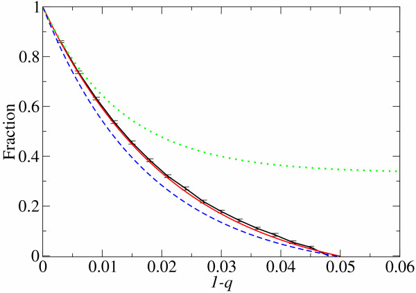
Figure 3 Comparison of population structure between analytical predictions and computer simulations The fraction of the fittest phenotype population is plotted against the error rate per base (1 - q). The black line (the solid line with error bars) is obtained from computer simulations. The red line (the solid line without error bars) is calculated with the additive assumption from Eq. 1 and Eq. 2 with σ = 10 and N = 76 as in the simulations. λ is set to be 0.4 which is the time averaged representative λ value observed in the simulations after the population evolves (see the Methods section – Non-uniform distribution of λ – for the definition of the representative λ). The green line (the dotted line) is obtained from the formulation of Reidys et al. [5] with the same parameters as the above. The blue line (the dashed line) is calculated with the four λ approximation by using λ values reported in [5] (λ = 0.2489 on average) and σ = 10 and N = 76 as in our simulations.
Figure 3 Comparison of population structure between analytical predictions and computer simulations The fraction of the fittest phenotype population is plotted against the error rate per base (1 - q). The black line (the solid line with error bars) is obtained from computer simulations. The red line (the solid line without error bars) is calculated with the additive assumption from Eq. 1 and Eq. 2 with σ = 10 and N = 76 as in the simulations. λ is set to be 0.4 which is the time averaged representative λ value observed in the simulations after the population evolves (see the Methods section – Non-uniform distribution of λ – for the definition of the representative λ). The green line (the dotted line) is obtained from the formulation of Reidys et al. [5] with the same parameters as the above. The blue line (the dashed line) is calculated with the four λ approximation by using λ values reported in [5] (λ = 0.2489 on average) and σ = 10 and N = 76 as in our simulations.CC BY · PubMed Central
Figure 4 Number of substitutions per replication in mutants The y-axis is the number of base substitutions (d) per replication (or per neutral replication) at the error threshold. The thick solid line represents the average d per neutral replication (i.e., the average d of the sequences which retain the master phenotype per replication): d = Np/(qmim + p) where p = λ (1 - qmin) and λ = (σ-1/N - qmin)/(1 - qmin). The thin solid line represents the standard deviation of it, i.e., ± (qmim + p) Np . The dashed line represents the average d per replication, which is N(1 - qmin). N is 100 and σ is 10. The lines are plotted against qmin (the lower x-axis), and the corresponding λ is shown in the upper x-axis.
Figure 4 Number of substitutions per replication in mutants The y-axis is the number of base substitutions (d) per replication (or per neutral replication) at the error threshold. The thick solid line represents the average d per neutral replication (i.e., the average d of the sequences which retain the master phenotype per replication): d = Np/(qmim + p) where p = λ (1 - qmin) and λ = (σ-1/N - qmin)/(1 - qmin). The thin solid line represents the standard deviation of it, i.e., ± (qmim + p) Np . The dashed line represents the average d per replication, which is N(1 - qmin). N is 100 and σ is 10. The lines are plotted against qmin (the lower x-axis), and the corresponding λ is shown in the upper x-axis.CC BY · PubMed Central
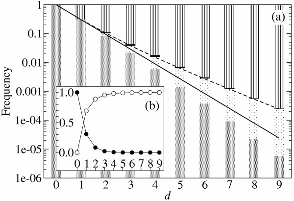
Figure 5 Additivity and epistasis in RNA folding The frequency of mutant classes is plotted against the number of base substitutions (d). (a) Log. plot. The patterns in the bars indicate the mutant classes: (from bottom) mesh, additive neutral; dots, positive epistasis; black, negative epistasis; stripes, additive deleterious (see Table 1 for the definition). The data were generated by RNA folding (by using [7]) with a S. cerevisiae tRNAphe sequence as a reference sequence: GCGGAUUUACCUCAGUUGGGAGAGGGCCAGACUGAACAUCUGGAGGUCCGGCGCGCGAUACGCCGAAUUCGCACCA (each non-RNA is converted to RNA). We examined all possible mutants at d = 1, 2 and the subsets of mutants for other d values (2<d<10, the portion of examined mutants is respectively, 10, 1, 0.1, 0.01, 0.3 × 10⁻³, 0.1 × 10⁻³, 0.4 × 10⁻⁵%). These observations in RNA folding are compared with the following two analytical predictions. The solid line is the probability of neutral replication estimated under the additive assumption (λd, λ = 0.307). The dashed line is the probability of neutral replication estimated with epistasis ((d), see Methods section – Probabilistic approach). (b) Linear plot. Symbols: ● the frequency of the neutral mutants (additive neutral and positive epistasis); ○ the frequency of the deleterious mutants (additive deleterious and negative epistasis).
Figure 5 Additivity and epistasis in RNA folding The frequency of mutant classes is plotted against the number of base substitutions (d). (a) Log. plot. The patterns in the bars indicate the mutant classes: (from bottom) mesh, additive neutral; dots, positive epistasis; black, negative epistasis; stripes, additive deleterious (see Table 1 for the definition). The data were generated by RNA folding (by using [7]) with a S. cerevisiae tRNAphe sequence as a reference sequence: GCGGAUUUACCUCAGUUGGGAGAGGGCCAGACUGAACAUCUGGAGGUCCGGCGCGCGAUACGCCGAAUUCGCACCA (each non-RNA is converted to RNA). We examined all possible mutants at d = 1, 2 and the subsets of mutants for other d values (2<d<10, the portion of examined mutants is respectively, 10, 1, 0.1, 0.01, 0.3 × 10⁻³, 0.1 × 10⁻³, 0.4 × 10⁻⁵%). These observations in RNA folding are compared with the following two analytical predictions. The solid line is the probability of neutral replication estimated under the additive assumption (λd, λ = 0.307). The dashed line is the probability of neutral replication estimated with epistasis ((d), see Methods section – Probabilistic approach). (b) Linear plot. Symbols: ● the frequency of the neutral mutants (additive neutral and positive epistasis); ○ the frequency of the deleterious mutants (additive deleterious and negative epistasis).CC BY · PubMed Central
Figure 6 Comparison between additivity and epistasis in RNA folding (a) The relative probability of neutral replication under the additive assumption (λd) is plotted against the number of base substitutions (d), where the probability of neutral replication with epistasis (i.e. the fraction of neutral mutants observed in the yeast tRNAphe folding) is set to be 1 for each d as a reference. It can be seen that the effect of epistasis on the probability of neutral replication becomes larger as the number of substitution (d) increases. The same data as that of Fig. 5 are used. (b) The solid line (the left y-axis) represents the relative effective replication accuracy (Qe) under the additive assumption plotted against the error rate (1 - q), where Qe calculated with epistasis is set to be 1 as reference (see Methods section – Probabilistic approach – for details). It can be seen that the effect of epistasis on Qe increases as the error rate (1 - q) increases. The shape of the curve is in a similar manner as that of the curve in Fig 6a. Although the x-axis of Fig 6b is different from that of Fig 6a, one can relate the two graphs via the average d per neutral replication, with which the different x-axes can be transformed to each other. The average d per neutral replication is represented by the dashed line (the right y-axis plotted against 1 - q). Its value is calculated under the additive assumption as d = Np/(q + p) where p = λ (1 - q), λ = 0.4 and N = 76.
Figure 6 Comparison between additivity and epistasis in RNA folding (a) The relative probability of neutral replication under the additive assumption (λd) is plotted against the number of base substitutions (d), where the probability of neutral replication with epistasis (i.e. the fraction of neutral mutants observed in the yeast tRNAphe folding) is set to be 1 for each d as a reference. It can be seen that the effect of epistasis on the probability of neutral replication becomes larger as the number of substitution (d) increases. The same data as that of Fig. 5 are used. (b) The solid line (the left y-axis) represents the relative effective replication accuracy (Qe) under the additive assumption plotted against the error rate (1 - q), where Qe calculated with epistasis is set to be 1 as reference (see Methods section – Probabilistic approach – for details). It can be seen that the effect of epistasis on Qe increases as the error rate (1 - q) increases. The shape of the curve is in a similar manner as that of the curve in Fig 6a. Although the x-axis of Fig 6b is different from that of Fig 6a, one can relate the two graphs via the average d per neutral replication, with which the different x-axes can be transformed to each other. The average d per neutral replication is represented by the dashed line (the right y-axis plotted against 1 - q). Its value is calculated under the additive assumption as d = Np/(q + p) where p = λ (1 - q), λ = 0.4 and N = 76.CC BY · PubMed Central
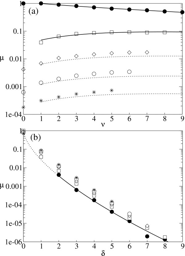
Figure 7 Probabilistic approach in calculating the effective replication accuracy with epistasis (a) The probability that a mutant is neutral with v neutral substitutions and δ deleterious substitutions (i.e., μ(v, δ)) is plotted against the number of neutral substitutions (v). Symbols: ● δ = 0; □ δ = 1; ◇ δ = 2; ○ δ = 3; * δ = 4. The plots were obtained from the same data set as that of Fig. 5. The solid lines represent the results of curve fitting. We used Eq. 10 (v>0, δ = 0) to the δ = 0 data set, and Eq. 10 (v>0, δ>0) to the δ = 1 data set. The second fitting was done after we obtained α and εn from the first fitting, and εd and η from the fitting in Fig. 7b. The dotted lines are the estimation made with the obtained parameters (listed below). (b) μ(v, δ) plotted against the number of deleterious substitutions (δ). Symbols: ● v = 0; □ v = 1; ◇ v = 2; ○ v = 3; * v = 4. The solid part of the line represents the curve fitting; the dotted part is an exception, i.e., μ(0, 1) = 0. We used Eq. 10 (v = 0, δ>0) toward the v = 0 data set in the fitting. All the fitting was done after transforming both the equations and the data sets to logarithmic scale to reduce the biased importance of the points in small d. The obtained parameters are as follows: εn = 0.1190, α = 0.8483, εnd = 2.418, β = 2.333, γ = 3.996, εd = 0.02697 and η = 0.6380.
Figure 7 Probabilistic approach in calculating the effective replication accuracy with epistasis (a) The probability that a mutant is neutral with v neutral substitutions and δ deleterious substitutions (i.e., μ(v, δ)) is plotted against the number of neutral substitutions (v). Symbols: ● δ = 0; □ δ = 1; ◇ δ = 2; ○ δ = 3; * δ = 4. The plots were obtained from the same data set as that of Fig. 5. The solid lines represent the results of curve fitting. We used Eq. 10 (v>0, δ = 0) to the δ = 0 data set, and Eq. 10 (v>0, δ>0) to the δ = 1 data set. The second fitting was done after we obtained α and εn from the first fitting, and εd and η from the fitting in Fig. 7b. The dotted lines are the estimation made with the obtained parameters (listed below). (b) μ(v, δ) plotted against the number of deleterious substitutions (δ). Symbols: ● v = 0; □ v = 1; ◇ v = 2; ○ v = 3; * v = 4. The solid part of the line represents the curve fitting; the dotted part is an exception, i.e., μ(0, 1) = 0. We used Eq. 10 (v = 0, δ>0) toward the v = 0 data set in the fitting. All the fitting was done after transforming both the equations and the data sets to logarithmic scale to reduce the biased importance of the points in small d. The obtained parameters are as follows: εn = 0.1190, α = 0.8483, εnd = 2.418, β = 2.333, γ = 3.996, εd = 0.02697 and η = 0.6380.CC BY · PubMed Central

Verification

Claims the paper makes

The claims and statistics of this paper haven’t been checked yet.

Free: it reads the open-access text and checks the first 5 claims that cite a source we can check. Create a free account to check every claim.

A few free checks a day · papers already verified open instantly · results are public

Self-check

Percentages, sums and reported differences re-computed from the paper’s own numbers.

The self-check needs the paper’s full text.

Citations

Cites

Show all 14 references

Cited by

See all 54

Metadata

Authors
Takeuchi, N., Poorthuis, P. H., & Hogeweg, P.
Affiliations
Utrecht University (NL)
Corresponding author
Takeuchi, Nobuto
Venue
BMC Evolutionary Biology
Published
2005-02-03
Volume
5
Issue
1
Pages
9-9
ISSN
1471-2148 (ISSN-L)
OpenAlex
W2144107393
Cited by
54
References
14
Citations by year
2026: 1 · 2021: 3 · 2020: 3 · 2019: 3 · 2018: 2 · 2017: 1 · 2016: 2 · 2015: 2 · 2014: 4 · 2013: 3 · 2012: 4
FWCI
2.16
Type
journal article
Language
en
Open access
Licence
Locations
  • BMC Evolutionary Biology (publishedVersion, cc-by)
  • PubMed Central (publishedVersion, cc-by)
  • PubMed (publishedVersion)
  • DOAJ (DOAJ: Directory of Open Access Journals) (submittedVersion, cc-by-sa)
Topics
  • Life Sciences › Biochemistry, Genetics and Molecular Biology › Genetics › Evolution and Genetic Dynamics
  • Life Sciences › Biochemistry, Genetics and Molecular Biology › Molecular Biology › RNA and protein synthesis mechanisms
  • Physical Sciences › Physics and Astronomy › Astronomy and Astrophysics › Origins and Evolution of Life
Keywords
genotype-phenotype mapping, epistasis, additivity, RNA evolution, RNA folding, base substitutions
MeSH terms
Algorithms, Computer Simulation, Epistasis, Genetic, Genotype, Models, Genetic, Mutation, Nucleic Acid Conformation, Phenotype, Probability, RNA, Software, Reproducibility of Results, Models, Statistical, Evolution, Molecular, Computational Biology, Genomics

About these checks

Registry, retraction, Cites and statistics results are computed, not judged, with one exception: a printed reference that no index lists is read once by a model before it counts as a citation error. Claims are extracted by a model and kept only when their quote appears verbatim in the text; each cited source is then checked, with a model’s help, for whether it says what the claim relies on. Those verdicts can be wrong — read the claim’s quote and the cited source before relying on one.

Statistics and arithmetic are recomputed, not judged.

Confidence bands are shown only for fields calibrated on our annotated test set. None is calibrated yet, so no band is shown.

What counts as a claim ›How we measure confidence ›How we check this ›

Are you an author, or do you see a problem with this page? Request a review

How to cite

Cite CoChat for the checks on this page, and the paper for its own findings.

This page
CoChat. (2026). Citation check: Phenotypic error threshold; additivity and epistasis in RNA evolution. https://app.cochat.ai/papers/10.1186/1471-2148-5-9
The paper
Takeuchi, N., Poorthuis, P. H., & Hogeweg, P. (2005). Phenotypic error threshold; additivity and epistasis in RNA evolution. BMC Evolutionary Biology. https://doi.org/10.1186/1471-2148-5-9

Data sources

Bibliographic data: Semantic Scholar, OpenAlex, Crossref.

Contains information from the Semantic Scholar Academic Graph Datasets, made available under the ODC Attribution License (ODC-BY 1.0).

Semantic Scholar’s data is described in: Kinney, R., et al. (2023). The Semantic Scholar Open Data Platform. arXiv:2301.10140.