

The DOI matches its Crossref record; 108 of the 111 references it cites were found in a registry or an index.
Meta-evaluation of meta-analysis: ten appraisal questions for biologists
Open accessAbstract
Meta-analysis is a statistical procedure for analyzing the combined data from different studies, and can be a major source of concise up-to-date information. The overall conclusions of a meta-analysis, however, depend heavily on the quality of the meta-analytic process, and an appropriate evaluation of the quality of meta-analysis (meta-evaluation) can be challenging. We outline ten questions biologists can ask to critically appraise a meta-analysis. These questions could also act as simple and accessible guidelines for the authors of meta-analyses. We focus on meta-analyses using non-human species, which we term 'biological' meta-analysis. Our ten questions are aimed at enabling a biologist to evaluate whether a biological meta-analysis embodies 'mega-enlightenment', a 'mega-mistake', or something in between.
Overview
The claims and statistics of this paper haven’t been checked yet.
Run the check — free, no account needed. It reads the open-access text and checks the sources it cites.
Integrity signals
Registry
Cites
Statistics
Figures
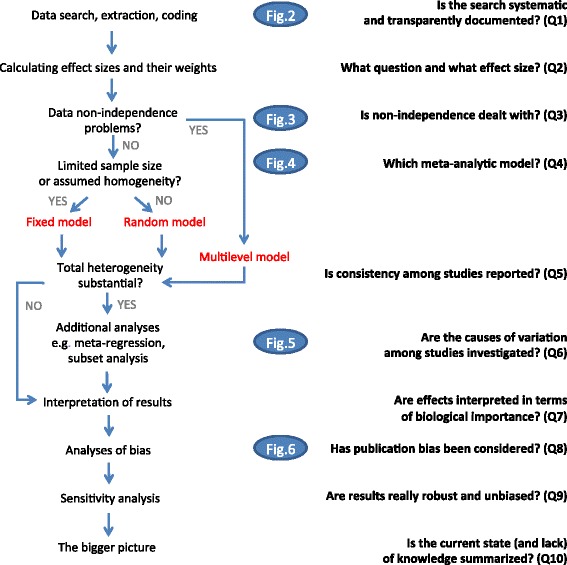
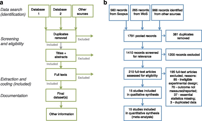
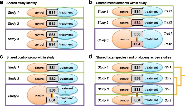
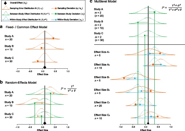
Verification
Claims the paper makes
The claims and statistics of this paper haven’t been checked yet.
Run the check — free, no account needed. It reads the open-access text and checks the sources it cites.
Claims other papers make about this one
Each is checked against this paper’s own text: does it say what the citing paper says it does?
The cited source says what the claim attributes to it.
In the citing paper
“This bias, known as publication bias, can be mitigated by gathering the most comprehensive database possible (Lortie et al., 2007; Nakagawa et al., 2017).”
From Acoustic indices as proxies for biodiversity: a meta‐analysis (2022) · cites this paper as Nakagawa et al., 2017
In the citing paper
“since poorly and inexpertly conducted meta-analyses can provide biased and misleading results (24, 32).”
From Agricultural diversification promotes multiple ecosystem services without compromising yield (2020) · cites this paper as [32]
In the citing paper
“While the number of published meta-analyses has continued to increase rapidly within and among disciplines, too many meta-analyses are of low quality 13-15 .”
From Meta-analysis and the science of research synthesis (2018) · cites this paper as [15]
Self-check
Percentages, sums and reported differences re-computed from the paper’s own numbers.
The self-check needs the paper’s full text.
Citations
Cites
Preferred Reporting Items for Systematic Reviews and Meta-Analyses: the PRISMA statement
Moher, D., Liberati, A., Tetzlaff, J., Altman, D. G., & for the PRISMA Group (2009) · BMJ · doi:10.1136/bmj.b2535 · Cited by 83,823
Measuring inconsistency in meta-analyses
Higgins, J. P. T., Thompson, S. G., Deeks, J. J., & Altman, D. G. (2003) · BMJ · doi:10.1136/bmj.327.7414.557 · Cited by 63,139
Bias in meta-analysis detected by a simple, graphical test
Egger, M., Smith, G. D., Schneider, M., & Minder, C. (1997) · BMJ · doi:10.1136/bmj.315.7109.629 · Cited by 56,722
Preferred reporting items for systematic reviews and meta-analyses: the PRISMA Statement.
(2009) · PubMed Central · Cited by 44,859
Preferred reporting items for systematic reviews and meta-analyses: The PRISMA statement
Moher, D., Liberati, A., Tetzlaff, J., Altman, D. G., & the PRISMA Group* (2009) · Annals of Internal Medicine · doi:10.7326/0003-4819-151-4-200908180-00135 · Cited by 37,554
Quantifying heterogeneity in a meta‐analysis
Higgins, J. P. T., & Thompson, S. G. (2002) · Statistics in Medicine · doi:10.1002/sim.1186 · Cited by 36,763
Liberati, A., Altman, D. G., Tetzlaff, J., Mulrow, C., Gøtzsche, P. C., Ioannidis, J. P. A., Clarke, M., Devereaux, P. J., Kleijnen, J., & Moher, D. (2009) · PLoS Medicine · doi:10.1371/journal.pmed.1000100 · Cited by 28,164
Cochrane Handbook for Systematic Reviews of Interventions: Cochrane Book Series
(2008) · doi:10.1002/9780470712184 · Cited by 25,048
Conducting Meta-Analyses in R with the metafor Package
Viechtbauer, W. (2010) · Journal of Statistical Software · doi:10.18637/jss.v036.i03 · Cited by 20,464
Borenstein, M., Hedges, L. V., Higgins, J. P. T., & Rothstein, H. R. (2009) · doi:10.1002/9780470743386 · Cited by 14,225
Research works printed but not linked: 10
- Hedges L, Olkin I. Statistical methods for meta-analysis. New York: Academic Press; 1985.
- Nakagawa S, Kubo T. Statistical models for meta-analysis in ecology and evolution (in Japanese). Proc Inst Stat Math. 2016;64(1):105–21.
- Borenstein M. Effect size for continuous data. In: Cooper H, Hedges LV, Valentine JC, editors. The handbook of research synthesis and meta-analysis. New York: Russell Sage Foundation; 2009. p. 221–35.
- Fleiss JL, Berlin JA. Effect sizes for dichotomous data. In: Cooper H, Hedges LV, Valentine JC, editors. The handbook of research synthesis and meta-analysis. New York: Russell Sage Foundation; 2009. p. 237–53.
- Rosenberg MS, Adams DC, Gurevitch J. MetaWin: statistical software for meta-analysis. 2nd ed. Sunderland: Sinauer; 2000.
- Lajeunesse MJ. Meta-analysis and the comparative phylogenetic method. Am Nat. 2009;174:369–81. · DOI
- Vetter D, Rucker G, Storch I. Meta-analysis: a need for well-defined usage in ecology and conservation biology. Ecosphere. 2013;4(6):1–24. · DOI
- Higgins JPT, Green S. Cochrane handbook for systematic reviews of interventions. West Sussex: Wiley-Blackwell; 2009.
- Cohen J. Statistical power analysis for the beahvioral sciences. 2nd ed. Hillsdale: Lawrence Erlbaum; 1988.
- Sutton AJ. Publication bias. In: Cooper H, Hedges L, Valentine J, editors. The handbook of research synthesis and meta-analysis. New York: Russell Sage Foundation; 2009. p. 435–52.
Cited by
Sorted by citations
Meta-analysis and the science of research synthesis
Gurevitch, J., Koricheva, J., Nakagawa, S., & Stewart, G. (2018) · Nature · doi:10.1038/nature25753 · Cited by 1,709
Self-citationAgricultural diversification promotes multiple ecosystem services without compromising yield
Tamburini, G., Bommarco, R., Wanger, T. C., Kremen, C., van der Heijden, M. G. A., Liebman, M., & Hallin, S. (2020) · Science Advances · doi:10.1126/sciadv.aba1715 · Cited by 1,110
O’Dea, R. E., Lagisz, M., Jennions, M. D., Koricheva, J., Noble, D. W. A., Parker, T. H., Gurevitch, J., Page, M. J., Stewart, G. B., Moher, D., et al. (2021) · Biological reviews/Biological reviews of the Cambridge Philosophical Society · doi:10.1111/brv.12721 · Cited by 825
Self-citationPositive but variable effects of crop diversification on biodiversity and ecosystem services
Beillouin, D., Ben‐Ari, T., Malézieux, E., Seufert, V., & Makowski, D. (2021) · Global Change Biology · doi:10.1111/gcb.15747 · Cited by 590
PD-L1 expression by dendritic cells is a key regulator of T-cell immunity in cancer
Oh, S. A., Wu, D.-C., Cheung, J., Navarro, A., Xiong, H., Cubas, R. A., Tótpál, K., Chiu, H. H., Wu, Y., Comps‐Agrar, L., et al. (2020) · Nature Cancer · doi:10.1038/s43018-020-0075-x · Cited by 466
Methods for testing publication bias in ecological and evolutionary meta‐analyses
Nakagawa, S., Lagisz, M., Jennions, M. D., Koricheva, J., Noble, D. W. A., Parker, T. H., Sánchez‐Tójar, A., Yang, Y., & O'Dea, R. E. (2022) · Methods in Ecology and Evolution · doi:10.1111/2041-210x.13724 · Cited by 399
Self-citationA global synthesis of biodiversity responses to glacier retreat
Cauvy-Fraunié, S., & Dangles, O. (2019) · Nature Ecology & Evolution · doi:10.1038/s41559-019-1042-8 · Cited by 337
Loh, R., Stamatakis, E., Folkerts, D., Allgrove, J. E., & Moir, H. J. (2020) · Sports Medicine · doi:10.1007/s40279-019-01183-w · Cited by 326
Biodiversity promotes ecosystem functioning despite environmental change
Hong, P., Schmid, B., Laender, F. D., Eisenhauer, N., Zhang, X., Chen, H., Craven, D., Boeck, H. J. D., Hautier, Y., Petchey, O. L., et al. (2021) · Ecology Letters · doi:10.1111/ele.13936 · Cited by 365
Mijatovic-Vukas, J., Capling, L., Cheng, S., Stamatakis, E., Louie, J., Cheung, N. W., Markovic, T., Ross, G., Senior, A., Brand-Miller, J. C., et al. (2018) · Nutrients · doi:10.3390/nu10060698 · Cited by 315
Self-citationThe pervasive and multifaceted influence of biocrusts on water in the world's drylands
Eldridge, D. J., Reed, S. C., Travers, S. K., Bowker, M. A., Maestre, F. T., Ding, J., Havrilla, C. A., Rodríguez‐Caballero, E., Barger, N. N., Weber, B., et al. (2020) · Global Change Biology · doi:10.1111/gcb.15232 · Cited by 317
Noble, D. W. A., Stenhouse, V., & Schwanz, L. E. (2017) · Biological reviews/Biological reviews of the Cambridge Philosophical Society · doi:10.1111/brv.12333 · Cited by 305
Self-citationA meta-analysis of the ecological and economic outcomes of mangrove restoration
Su, J., Friess, D. A., & Gasparatos, A. (2021) · Nature Communications · doi:10.1038/s41467-021-25349-1 · Cited by 316
Global effects of non‐native tree species on multiple ecosystem services
Castro‐Díez, P., Vaz, A. S., Silva, J. S., van Loo, M., Alonso, Á., Aponte, C., Bayón, Á., Bellingham, P. J., Chiuffo, M. C., DiManno, N., et al. (2019) · Biological Reviews · doi:10.1111/brv.12511 · Cited by 281
Acoustic indices as proxies for biodiversity: a meta‐analysis
Alcocer, I., Lima, H., Sugai, L. S. M., & Llusia, D. (2022) · Biological Reviews · doi:10.1111/brv.12890 · Cited by 273
“This bias, known as publication bias, can be mitigated by gathering the most comprehensive database possible (Lortie et al., 2007; Nakagawa et al., 2017).”
BackgroundTree Diversity and Forest Resistance to Insect Pests: Patterns, Mechanisms, and Prospects
Jactel, H., Moreira, X., & Castagneyrol, B. (2020) · Annual Review of Entomology · doi:10.1146/annurev-ento-041720-075234 · Cited by 296
Nonindependence and sensitivity analyses in ecological and evolutionary meta‐analyses
Noble, D. W. A., Lagisz, M., O’Dea, R. E., & Nakagawa, S. (2017) · Molecular Ecology · doi:10.1111/mec.14031 · Cited by 273
Self-citationResearch Weaving: Visualizing the Future of Research Synthesis
Nakagawa, S., Samarasinghe, G., Haddaway, N., Westgate, M. J., O’Dea, R. E., Noble, D. W. A., & Lagisz, M. (2018) · Trends in Ecology & Evolution · doi:10.1016/j.tree.2018.11.007 · Cited by 278
Self-citationSchlaepfer, D. R., Braschler, B., Rusterholz, H., & Baur, B. (2018) · Ecosphere · doi:10.1002/ecs2.2488 · Cited by 270
Global variation in soil carbon sequestration potential through improved cropland management
Lessmann, M., Ros, G. H., Young, M. D., & VRIES, W. D. (2021) · Global Change Biology · doi:10.1111/gcb.15954 · Cited by 274
The orchard plot: Cultivating a forest plot for use in ecology, evolution, and beyond
Nakagawa, S., Lagisz, M., O’Dea, R. E., Rutkowska, J., Yang, Y., Noble, D. W. A., & Senior, A. M. (2020) · Research Synthesis Methods · doi:10.1002/jrsm.1424 · Cited by 217
Self-citationPositive biodiversity–productivity relationships in forests: climate matters
Jactel, H., Gritti, E., Drößler, L., Forrester, D. I., Mason, W. L., Morin, X., Pretzsch, H., & Castagneyrol, B. (2018) · Biology Letters · doi:10.1098/rsbl.2017.0747 · Cited by 232
The positive impact of conservation action
Langhammer, P. F., Bull, J. W., Bicknell, J. E., Oakley, J. L., Brown, M. H., Bruford, M. W., Butchart, S. H. M., Carr, J., Church, D., Cooney, R., et al. (2024) · Science · doi:10.1126/science.adj6598 · Cited by 246
Nakagawa, S., Yang, Y., Macartney, E. L., Spake, R., & Lagisz, M. (2023) · Environmental Evidence · doi:10.1186/s13750-023-00301-6 · Cited by 242
Self-citationEvidence that organic farming promotes pest control
Muneret, L., Mitchell, M. G. E., Seufert, V., Aviron, S., Djoudi, E. A., Pétillon, J., Plantegenest, M., Thiéry, D., & Rusch, A. (2018) · Nature Sustainability · doi:10.1038/s41893-018-0102-4 · Cited by 219
Johnson, B. T., & Hennessy, E. A. (2019) · Social Science & Medicine · doi:10.1016/j.socscimed.2019.05.035 · Cited by 238
Galkanda‐Arachchige, H. S. C., Wilson, A. E., & Davis, D. A. (2019) · Reviews in Aquaculture · doi:10.1111/raq.12401 · Cited by 190
Cardinale, B. J., Gonzalez, A., Allington, G. R. H., & Loreau, M. (2018) · Biological Conservation · doi:10.1016/j.biocon.2017.12.021 · Cited by 190
The effects of anthropogenic noise on animals: a meta-analysis
Kunc, H. P., & Schmidt, R. (2019) · Biology Letters · doi:10.1098/rsbl.2019.0649 · Cited by 196
Phenolic Compound Induction in Plant-Microbe and Plant-Insect Interactions: A Meta-Analysis
Wallis, C. M., & Galarneau, E. (2020) · Frontiers in Plant Science · doi:10.3389/fpls.2020.580753 · Cited by 178
Quantifying the impacts of defaunation on natural forest regeneration in a global meta-analysis
Gardner, C. J., Bicknell, J. E., Baldwin-Cantello, W., Struebig, M. J., & Davies, Z. G. (2019) · Nature Communications · doi:10.1038/s41467-019-12539-1 · Cited by 189
A mother’s legacy: the strength of maternal effects in animal populations
Moore, M. P., Whiteman, H. H., & Martin, R. A. (2019) · Ecology Letters · doi:10.1111/ele.13351 · Cited by 176
Tetzlaff, S. J., Sperry, J., & DeGregorio, B. (2019) · Biological Conservation · doi:10.1016/j.biocon.2019.05.054 · Cited by 157
The repeatability of cognitive performance: a meta-analysis
Cauchoix, M., Chow, P. K. Y., van Horik, J. O., Atance, C. M., Barbeau, E. J., Barragan‐Jason, G., Bize, P., Boussard, A., Buechel, S. D., Cabirol, A., et al. (2018) · Philosophical Transactions of the Royal Society B Biological Sciences · doi:10.1098/rstb.2017.0281 · Cited by 164
Self-citationEffect of the plastic pollutant bisphenol A on the biology of aquatic organisms: A meta‐analysis
Wu, N. C., & Seebacher, F. (2020) · Global Change Biology · doi:10.1111/gcb.15127 · Cited by 168
Frontiers in quantifying wildlife behavioural responses to chemical pollution
Bertram, M. G., Martin, J. M., McCallum, E. S., Alton, L. A., Brand, J. A., Brooks, B. W., Červený, D., Fick, J. B., Ford, A. T., Hellström, G., et al. (2022) · Biological reviews/Biological reviews of the Cambridge Philosophical Society · doi:10.1111/brv.12844 · Cited by 172
Self-citationMugwanya, M., Dawood, M. A. O., Kimera, F., & Sewilam, H. (2022) · Reviews in Aquaculture · doi:10.1111/raq.12701 · Cited by 159
Global occurrence, drivers, and environmental risks of microplastics in marine environments
Tang, L., Feng, J., Li, C., Liang, J., Zhang, S., & Yang, Z. (2022) · Journal of Environmental Management · doi:10.1016/j.jenvman.2022.116961 · Cited by 166
Seeds of future past: climate change and the thermal memory of plant reproductive traits
Fernández‐Pascual, E., Mattana, E., & Pritchard, H. W. (2018) · Biological reviews/Biological reviews of the Cambridge Philosophical Society · doi:10.1111/brv.12461 · Cited by 148
Meta-analytic evidence that sexual selection improves population fitness
Cally, J., Stuart-Fox, D. M., & Holman, L. (2019) · Nature Communications · doi:10.1038/s41467-019-10074-7 · Cited by 142
Mathot, K. J., Dingemanse, N., & Nakagawa, S. (2018) · Biological Reviews of The Cambridge Philosophical Society · doi:10.1111/brv.12491 · Cited by 123
Self-citationOvercompensation for insect herbivory: a review and meta‐analysis of the evidence
Garcia, L. C., & Eubanks, M. D. (2018) · Ecology · doi:10.1002/ecy.2585 · Cited by 133
Noble, D. W. A., Radersma, R., & Uller, T. (2019) · Proceedings of the National Academy of Sciences · doi:10.1073/pnas.1821066116 · Cited by 133
Self-citationGonzález, A. V., Gómez‐Silva, V., Ramírez, M. J., & Fontúrbel, F. E. (2019) · Conservation Biology · doi:10.1111/cobi.13422 · Cited by 131
Prevention not cure: a review of methods to avoid sea lice infestations in salmon aquaculture
Barrett, L. T., Oppedal, F., Robinson, N. A., & Dempster, T. (2020) · Reviews in Aquaculture · doi:10.1111/raq.12456 · Cited by 131
Global engineering effects of soil invertebrates on ecosystem functions
Wu, D., Du, E., Eisenhauer, N., Mathieu, J., & Chu, C. (2025) · Nature · doi:10.1038/s41586-025-08594-y · Cited by 132
Nakagawa, S., Noble, D. W. A., Lagisz, M., Spake, R., Viechtbauer, W., & Senior, A. M. (2022) · Ecology Letters · doi:10.1111/ele.14144 · Cited by 123
Self-citationBiochar addition reduces salinity in salt-affected soils with no impact on soil pH: A meta-analysis
Wang, X., Ding, J., Han, L., Tan, J., Ge, X., & Nan, Q. (2024) · Geoderma · doi:10.1016/j.geoderma.2024.116845 · Cited by 121
Tarka, M., Guenther, A., Niemelä, P. T., Nakagawa, S., & Noble, D. W. A. (2018) · Behavioral Ecology and Sociobiology · doi:10.1007/s00265-018-2534-2 · Cited by 118
Self-citationEffects of developmental stress on animal phenotype and performance: a quantitative review
Eyck, H. J. F., Buchanan, K. L., Crino, O. L., & Jessop, T. S. (2019) · Biological reviews/Biological reviews of the Cambridge Philosophical Society · doi:10.1111/brv.12496 · Cited by 116
Elrys, A. S., Wang, J., Meng, L., Zhu, Q., El-Sawy, M. M., Chen, Z., Tu, X., El‐Saadony, M. T., Zhang, Y., Zhang, J., et al. (2023) · Nature Food · doi:10.1038/s43016-023-00888-6 · Cited by 111
Autumn bird migration phenology: A potpourri of wind, precipitation and temperature effects
Haest, B., Hüppop, O., van de Pol, M., & Bairlein, F. (2019) · Global Change Biology · doi:10.1111/gcb.14746 · Cited by 107
Plasticity leaves a phenotypic signature during local adaptation
Radersma, R., Noble, D. W. A., & Uller, T. (2020) · Evolution Letters · doi:10.1002/evl3.185 · Cited by 113
Self-citationTemporal Instability of Evidence Base: A Threat to Policy Making?
Koricheva, J., & Kulinskaya, E. (2019) · Trends in Ecology & Evolution · doi:10.1016/j.tree.2019.05.006 · Cited by 106
Sexual dimorphism in trait variability and its eco-evolutionary and statistical implications
Zajitschek, S. R. K., Zajitschek, F., Bonduriansky, R., Brooks, R. C., Cornwell, W. K., Falster, D. S., Lagisz, M., Mason, J., Senior, A. M., Noble, D. W. A., et al. (2020) · eLife · doi:10.7554/elife.63170 · Cited by 107
Self-citationCrean, A. J., & Senior, A. M. (2019) · Obesity Reviews · doi:10.1111/obr.12827 · Cited by 101
Self-citationDifferential effects of forestry plantations on bird diversity: A global assessment
Castaño‐Villa, G. J., Varón, J. V. E., Guevara, G., Bohada‐Murillo, M., & Fontúrbel, F. E. (2019) · Forest Ecology and Management · doi:10.1016/j.foreco.2019.03.025 · Cited by 106
Cait, J., Cait, A., Scott, R. W., Winder, C. B., & Mason, G. J. (2022) · BMC Biology · doi:10.1186/s12915-021-01184-0 · Cited by 114
Effects of microplastics on the toxicity of co-existing pollutants to fish: A meta-analysis
Yuan, F., Chen, H., Ding, Y., Wang, Y., Liao, Q., Wang, T., Fan, Q., Feng, Z., Zhang, C., Fu, G., et al. (2023) · Water Research · doi:10.1016/j.watres.2023.120113 · Cited by 100
Global food nutrients analysis reveals alarming gaps and daunting challenges
Wang, X., Dou, Z., Feng, S., Zhang, Y., Ma, L., Zou, C., Bai, Z., Lakshmanan, P., Shi, X., Liu, D., et al. (2023) · Nature Food · doi:10.1038/s43016-023-00851-5 · Cited by 103
Global meta-analysis reveals differential effects of microplastics on soil ecosystem
Wan, L., Cheng, H. L., Liu, Y., Shen, Y., Liu, G., & Su, X. (2023) · The Science of The Total Environment · doi:10.1016/j.scitotenv.2023.161403 · Cited by 104
Meta-analysis challenges a textbook example of status signalling and demonstrates publication bias
Sánchez‐Tójar, A., Nakagawa, S., Sánchez-Fortún, M., Martin, D. A., Ramani, S., Girndt, A., Bókony, V., Kempenaers, B., Liker, A., Westneat, D. F., et al. (2018) · eLife · doi:10.7554/elife.37385 · Cited by 99
Self-citationRunquist, R. D. B., Gorton, A. J., Yoder, J. B., Deacon, N. J., Grossman, J. J., Kothari, S., Lyons, M. P., Sheth, S. N., Tiffin, P., & Moeller, D. A. (2019) · The American Naturalist · doi:10.1086/707322 · Cited by 94
A survey of gene expression meta-analysis: methods and applications
Toro‐Domínguez, D., Villatoro-García, J. A., Martorell‐Marugán, J., Montoya, Y. R., Alarcón-Riquelme, M. E., & Carmona‐Sáez, P. (2020) · Briefings in Bioinformatics · doi:10.1093/bib/bbaa019 · Cited by 102
Moreira, X., Abdala‐Roberts, L., & Castagneyrol, B. (2018) · Journal of Ecology · doi:10.1111/1365-2745.12987 · Cited by 93
Meta‐Analysis of Copper and Iron in Parkinson's Disease Brain and Biofluids
Genoud, S., Senior, A. M., Hare, D. J., & Double, K. L. (2019) · Movement Disorders · doi:10.1002/mds.27947 · Cited by 95
Self-citationEffects of nutrient limitation on sperm and seminal fluid: a systematic review and meta‐analysis
Macartney, E. L., Crean, A. J., Nakagawa, S., & Bonduriansky, R. (2019) · Biological reviews/Biological reviews of the Cambridge Philosophical Society · doi:10.1111/brv.12524 · Cited by 94
Self-citationThe effects of ants on pest control: a meta-analysis
Anjos, D. V., Tena, A., Junior, A. B. V., Carvalho, R. L., Torezan‐Silingardi, H. M., Del‐Claro, K., & Perfecto, I. (2022) · Proceedings of the Royal Society B Biological Sciences · doi:10.1098/rspb.2022.1316 · Cited by 93
Pharmacological manipulations of judgement bias: A systematic review and meta-analysis
Neville, V., Nakagawa, S., Zidar, J., Paul, E. S., Lagisz, M., Melissa Bateson, B., Løvlie, H., & Mendl, M. (2019) · Neuroscience & Biobehavioral Reviews · doi:10.1016/j.neubiorev.2019.11.008 · Cited by 95
Self-citationLowe, E. B., Groves, R. L., & Gratton, C. (2021) · Agriculture Ecosystems & Environment · doi:10.1016/j.agee.2020.107290 · Cited by 100
Meta-analyses of flipped classroom studies: A review of methodology
Hew, K. F., Bai, S., Dawson, P., & Lo, C. K. (2021) · Educational Research Review · doi:10.1016/j.edurev.2021.100393 · Cited by 118
Bird-mediated effects of pest control services on crop productivity: a global synthesis
Díaz‐Siefer, P., Olmos-Moya, N., Fontúrbel, F. E., Lavandero, B. I., Pozo, R. A., & Celis-Diez, J. L. (2021) · Journal of Pest Science · doi:10.1007/s10340-021-01438-4 · Cited by 90
A meta‐analysis of herbivore effects on plant attractiveness to pollinators
Moreira, X., Castagneyrol, B., Abdala‐Roberts, L., & Traveset, A. (2019) · Ecology · doi:10.1002/ecy.2707 · Cited by 86
Salvage logging effects on regulating ecosystem services and fuel loads
Leverkus, A. B., Gustafsson, L., Lindenmayer, D. B., Castro, J., Beñayas, J. M. R., Ranius, T., & Thorn, S. (2020) · Frontiers in Ecology and the Environment · doi:10.1002/fee.2219 · Cited by 85
Putman, B. J., & Tippie, Z. A. (2020) · Frontiers in Ecology and Evolution · doi:10.3389/fevo.2020.580745 · Cited by 86
Costs of territoriality: a review of hypotheses, meta-analysis, and field study
Ord, T. J. (2021) · Oecologia · doi:10.1007/s00442-021-05068-6 · Cited by 83
Effects of landscape changes on water quality: A global meta-analysis
Shi, X., Mao, D., Song, K., Xiang, H., Li, S., & Wang, Z. (2024) · Water Research · doi:10.1016/j.watres.2024.121946 · Cited by 94
A contrast of meta and metafor packages for meta‐analyses in R
Lortie, C. J., & Filazzola, A. (2020) · Ecology and Evolution · doi:10.1002/ece3.6747 · Cited by 82
Liu, X., Chen, L., Liu, M., García‐Guzmán, G., Gilbert, G. S., & Zhou, S. (2020) · Oikos · doi:10.1111/oik.07027 · Cited by 85
Biological invasions are a population‐level rather than a species‐level phenomenon
Haubrock, P. J., Soto, I., Ahmed, D. A., Ansari, A. R., Tarkan, A. S., Kurtul, I., Macêdo, R. L., Lázaro‐Lobo, A., Toutain, M., Parker, B., et al. (2024) · Global Change Biology · doi:10.1111/gcb.17312 · Cited by 84
Gender wage gap in China: a large meta-analysis
Iwasaki, I., & Ma, X. (2020) · Journal for Labour Market Research · doi:10.1186/s12651-020-00279-5 · Cited by 84
Kossmeier, M., Tran, U. S., & Voracek, M. (2020) · BMC Medical Research Methodology · doi:10.1186/s12874-020-0911-9 · Cited by 83
Consequences of multiple imputation of missing standard deviations and sample sizes in meta‐analysis
Kambach, S., Bruelheide, H., Gerstner, K., Gurevitch, J., Beckmann, M., & Seppelt, R. (2020) · Ecology and Evolution · doi:10.1002/ece3.6806 · Cited by 81
Auditory Distraction During Reading: A Bayesian Meta-Analysis of a Continuing Controversy
Vasilev, M. R., Kirkby, J. A., & Angele, B. (2018) · Perspectives on Psychological Science · doi:10.1177/1745691617747398 · Cited by 85
Increased secondary aerosol contribution and possible processing on polluted winter days in China
Wang, Y., Chen, J., Wang, Q., Qin, Q., Ye, J., Han, Y., Li, L., Wei, Z. H., Zhi, Q., Zhang, Y., et al. (2019) · Environment International · doi:10.1016/j.envint.2019.03.021 · Cited by 78
Relationships between plant–soil feedbacks and functional traits
Xi, N., Adler, P. B., Chen, D., Wu, H., Catford, J. A., van Bodegom, P. M., Bahn, M., Crawford, K. M., & Chu, C. (2021) · Journal of Ecology · doi:10.1111/1365-2745.13731 · Cited by 76
Environmental enrichment increases aquatic animal welfare: A systematic review and meta‐analysis
Zhang, Z., Gao, L., & Zhang, X. (2021) · Reviews in Aquaculture · doi:10.1111/raq.12641 · Cited by 74
López‐Bedoya, P. A., Bohada‐Murillo, M., Ángel-Vallejo, M. C., Audino, L. D., Davis, A. L. V., Gurr, G. M., & Noriega, J. A. (2022) · Journal of Applied Ecology · doi:10.1111/1365-2664.14167 · Cited by 80
Yin, M., Li, H., Bai, M., Liu, H., Chen, Z., Deng, J., Deng, S., Chuan, M., Vollaard, N. B. J., Little, J. P., et al. (2023) · Applied Physiology, Nutrition, and Metabolism · doi:10.1139/apnm-2023-0329 · Cited by 84
Ecosystem services provided by armadillos
Rodrigues, T. F., Mantellatto, A. M. B., Superina, M., & Chiarello, A. G. (2019) · Biological reviews/Biological reviews of the Cambridge Philosophical Society · doi:10.1111/brv.12551 · Cited by 75
Harrison, L. M., Noble, D. W. A., & Jennions, M. D. (2021) · Biological reviews/Biological reviews of the Cambridge Philosophical Society · doi:10.1111/brv.12818 · Cited by 79
Self-citationHaave‐Audet, E., Besson, A. A., Nakagawa, S., & Mathot, K. J. (2021) · Biological reviews/Biological reviews of the Cambridge Philosophical Society · doi:10.1111/brv.12819 · Cited by 75
Self-citationThe impacts of tropical agriculture on biodiversity: A meta‐analysis
Oakley, J. L., & Bicknell, J. E. (2022) · Journal of Applied Ecology · doi:10.1111/1365-2664.14303 · Cited by 72
Biochar dose-dependent impacts on soil bacterial and fungal diversity across the globe
Zhao, J., Qiu, Y., Yi, F., Li, J., Wang, X., Fu, Q., Fu, X., Yao, Z., Dai, Z., Qiu, Y., et al. (2024) · The Science of The Total Environment · doi:10.1016/j.scitotenv.2024.172509 · Cited by 66
How much does climate change add to the challenge of feeding the planet this century?
Aggarwal, P. K., Vyas, S., Thornton, P. K., & Campbell, B. (2018) · Environmental Research Letters · doi:10.1088/1748-9326/aafa3e · Cited by 74
Meta‐analysis of social science research: A practitioner's guide
Iršová, Z., Doucouliagos, H., Havránek, T., & Stanley, T. D. (2023) · Journal of Economic Surveys · doi:10.1111/joes.12595 · Cited by 76
Synthesizing the evidence of nitrous oxide mitigation practices in agroecosystems
Grados, D., Butterbach‐Bahl, K., Chen, J., van Groenigen, K. J., Olesen, J. E., van Groenigen, J. W., & Ábalos, D. (2022) · Environmental Research Letters · doi:10.1088/1748-9326/ac9b50 · Cited by 74
Sáez, A., Aguilar, R., Ashworth, L., Gleiser, G., Morales, C. L., Traveset, A., & Aizen, M. A. (2022) · Proceedings of the Royal Society B Biological Sciences · doi:10.1098/rspb.2022.0086 · Cited by 64
Improving quantitative synthesis to achieve generality in ecology
Spake, R., O’Dea, R., Nakagawa, S., Doncaster, C. P., Ryo, M., Callaghan, C., & Bullock, J. (2022) · Nature Ecology & Evolution · doi:10.1038/s41559-022-01891-z · Cited by 62
Self-citationGlobal Climate Change Increases Terrestrial Soil CH4 Emissions
Guo, J., Feng, H., Peng, C. H., Chen, H., Xu, X., Ma, X., Li, L., Kneeshaw, D., Ruan, H., Yang, H., et al. (2023) · Global Biogeochemical Cycles · doi:10.1029/2021gb007255 · Cited by 64
Metadata
- Authors
- Nakagawa, S., Noble, D. W. A., Senior, A. M., & Lagisz, M.
- Affiliations
- Garvan Institute of Medical Research (AU)
- UNSW Sydney (AU)
- The University of Sydney (AU)
- Corresponding author
- Nakagawa, Shinichi
- Venue
- BMC Biology
- Published
- 2017-03-03
- Volume
- 15
- Issue
- 1
- Pages
- 18-18
- ISSN
- 1741-7007 (ISSN-L)
- PMC
- PMC5336618
- OpenAlex
- W2593372779
- Cited by
- 579
- References
- 111
- Citations by year
- 2026: 84 · 2025: 74 · 2024: 71 · 2023: 66 · 2022: 77 · 2021: 50 · 2020: 64 · 2019: 44 · 2018: 37 · 2017: 12
- FWCI
- 10.65
- Type
- journal article
- Language
- en
- Open access
- gold
- doi.org
- Licence
- cc-by
- Locations
- BMC Biology (publishedVersion, cc-by)
- PubMed Central (publishedVersion, cc-by)
- PubMed (publishedVersion)
- UNSWorks (University of New South Wales, Sydney, Australia) (submittedVersion, cc-by-nc-nd)
- Funders
- University of New South Wales
- University of Sydney
- Australian Research Council (DE150101774, FT130100268)
- Topics
- Social Sciences › Decision Sciences › Statistics, Probability and Uncertainty › Meta-analysis and systematic reviews
- Social Sciences › Library and Information Sciences › scientometrics and bibliometrics research
- Social Sciences › Psychology › Experimental and Cognitive Psychology › Psychology Research and Bibliometrics
- Keywords
- meta-evaluation, meta-analysis quality, critical appraisal, non-human species
- MeSH terms
- Documentation, Humans, Models, Theoretical, Publications, Meta-Analysis as Topic, Publication Bias, Knowledge
About these checks
Registry, retraction, Cites and statistics results are computed, not judged, with one exception: a printed reference that no index lists is read once by a model before it counts as a citation error. Claims are extracted by a model and kept only when their quote appears verbatim in the text; each cited source is then checked, with a model’s help, for whether it says what the claim relies on. Those verdicts can be wrong — read the claim’s quote and the cited source before relying on one.
Statistics and arithmetic are recomputed, not judged.
Confidence bands are shown only for fields calibrated on our annotated test set. None is calibrated yet, so no band is shown.
What counts as a claim ›How we measure confidence ›How we check this ›
Are you an author, or do you see a problem with this page? Request a review
