

The DOI matches its Crossref record; 25 of the 25 references it cites were found in a registry or an index.
Students Are Rarely Independent: When, Why, and How to Use Random Effects in Discipline-Based Education Research
Open accessAbstract
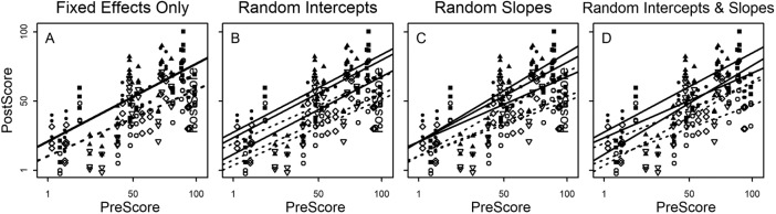
Discipline-based education researchers have a natural laboratory—classrooms, programs, colleges, and universities. Studies that administer treatments to multiple sections, in multiple years, or at multiple institutions are particularly compelling for two reasons: first, the sample sizes increase, and second, the implementation of the treatments can be intentionally designed and carefully monitored, potentially negating the need for additional control variables. However, when studies are implemented in this way, the observations on students are not completely independent; rather, students are clustered in sections, terms, years, or other factors. Here, I demonstrate why this clustering can be problematic in regression analysis. Fortunately, nonindependence of sampling can often be accounted for with random effects in multilevel regression models. Using several examples, including an extended example with R code, this paper illustrates why and how to implement random effects in multilevel modeling. It also provides resources to promote implementation of analyses that control for the nonindependence inherent in many quasi-random sampling designs.
Overview
The claims and statistics of this paper haven’t been checked yet.
Run the check — free, no account needed. It reads the open-access text and checks the sources it cites.
Integrity signals
Registry
Cites
Statistics
Figures
Verification
Claims the paper makes
The claims and statistics of this paper haven’t been checked yet.
Run the check — free, no account needed. It reads the open-access text and checks the sources it cites.
Claims other papers make about this one
Each is checked against this paper’s own text: does it say what the citing paper says it does?
The cited source says what the claim attributes to it.
In the citing paper
“We used hierarchical models to account for the nonindependence of student groups (MGS and non-MGS) from a single classroom (ref. 72 and SI Appendix).”
From Active learning narrows achievement gaps for underrepresented students in undergraduate science, technology, engineering, and math (2020) · cites this paper as [72]
Self-check
Percentages, sums and reported differences re-computed from the paper’s own numbers.
The self-check needs the paper’s full text.
Citations
Cites
Fitting Linear Mixed-Effects Models Using lme4
Bates, D., Mächler, M., Bolker, B., & Walker, S. (2015) · Journal of Statistical Software · doi:10.18637/jss.v067.i01 · Cited by 86,835
Model selection and multimodel inference: a practical information-theoretic approach.
Guthery, F. S., Burnham, K. P., & Anderson, D. R. (2003) · The Journal of Wildlife Management · doi:10.2307/3802723 · Cited by 41,495
Sample Selection Bias as a Specification Error
Heckman, J. J. (1979) · Econometrica · doi:10.2307/1912352 · Cited by 28,779
Mixed effects models and extensions in ecology with R
Zuur, A. F., Ieno, E. N., Walker, N., Saveliev, A. A., & Smith, G. M. (2009) · Statistics for Biology and Health · doi:10.1007/978-0-387-87458-6 · Cited by 17,963
Data Analysis Using Regression and Multilevel/Hierarchical Models
Gelman, A., & Hill, J. (2006) · doi:10.1017/cbo9780511790942 · Cited by 13,597
Active learning increases student performance in science, engineering, and mathematics
Freeman, S., Eddy, S. L., McDonough, M., Smith, M. K., Okoroafor, N., Jordt, H., & Wenderoth, M. P. (2014) · Proceedings of the National Academy of Sciences · doi:10.1073/pnas.1319030111 · Cited by 9,787
Generalized linear mixed models: a practical guide for ecology and evolution
Bolker, B. M., Brooks, M. E., Clark, C. J., Geange, S. W., Poulsen, J. R., Stevens, M. H. H., & White, J.-S. S. (2009) · Trends in Ecology & Evolution · doi:10.1016/j.tree.2008.10.008 · Cited by 8,910
The standards for educational and psychological testing.
Eignor, D. R. (2013) · American Psychological Association eBooks · doi:10.1037/14047-013 · Cited by 6,985
Standards for Educational and Psychological Testing
(2007) · Sage eBooks · doi:10.4135/9781412952644.n432 · Cited by 3,137
Discovering statistics using R
(2012) · Choice Reviews Online · doi:10.5860/choice.50-2114 · Cited by 2,548
Research works printed but not linked: 2
- R Core Team, 2017, A language and environment for statistical computing
- Rosenthal R., 1975, The volunteer subject
Cited by
Sorted by citations
Theobald, E. J., Hill, M. J., Tran, E., Agrawal, S., Arroyo, E. N., Behling, S., Chambwe, N., Cintrón, D. L., Cooper, J. D., Dunster, G., et al. (2020) · Proceedings of the National Academy of Sciences · doi:10.1073/pnas.1916903117 · Cited by 1,387
“A course-section random effect accounts for the nonindependence of observations on multiple students or student groups from each section from each course (72).”
Self-citationHarris, R. B., Mack, M. R., Bryant, J. R., Theobald, E. J., & Freeman, S. (2020) · Science Advances · doi:10.1126/sciadv.aaz5687 · Cited by 198
Self-citationEngland, B. J., Brigati, J. R., Schussler, E. E., & Musgrove, M. M. C. (2019) · CBE—Life Sciences Education · doi:10.1187/cbe.17-12-0284 · Cited by 142
Clemmons, A. W., Timbrook, J., Herron, J. C., & Crowe, A. J. (2020) · CBE—Life Sciences Education · doi:10.1187/cbe.19-11-0259 · Cited by 122
Energy savings and thermal comfort in a zero energy office building with fans in Singapore
Kent, M. G., Huynh, N. K., Mishra, A. K., Tartarini, F., Lipczyńska, A., Li, J., Sultan, Z., Goh, E., Karunagaran, G., Natarajan, A., et al. (2023) · Building and Environment · doi:10.1016/j.buildenv.2023.110674 · Cited by 103
Metadata
- Authors
- Theobald, E.
- Affiliations
- University of Washington (US)
- Corresponding author
- Theobald, Elli
- ORCID
- Theobald, Elli
- Venue
- CBE—Life Sciences Education
- Published
- 2018-09
- Volume
- 17
- Issue
- 3
- Pages
- rm2
- ISSN
- 1931-7913 (ISSN-L)
- PMC
- PMC6234830
- OpenAlex
- W2888039885
- Cited by
- 114
- References
- 25
- Citations by year
- 2026: 11 · 2025: 13 · 2024: 15 · 2023: 17 · 2022: 16 · 2021: 23 · 2020: 9 · 2019: 9 · 2018: 1
- FWCI
- 8.71
- Type
- journal article
- Language
- en
- Open access
- hybrid
- doi.org
- Licence
- cc-by-nc-sa
- Locations
- CBE—Life Sciences Education (publishedVersion, cc-by-nc-sa)
- Europe PMC (PubMed Central) (publishedVersion, cc-by-nc-sa)
- PubMed Central (publishedVersion, cc-by-nc-sa)
- PubMed (publishedVersion)
- Funders
- University of Washington
- Topics
- Physical Sciences › Mathematics › Statistics and Probability › Statistical Methods and Bayesian Inference
- Physical Sciences › Mathematics › Statistics and Probability › Statistics Education and Methodologies
- Social Sciences › Education › Educational Research and Methods
- Keywords
- random effects, multilevel regression, student clustering, treatment implementation, discipline-based education research
- MeSH terms
- Humans, Random Allocation, Research Design, Science, Students, Cluster Analysis, Multilevel Analysis
About these checks
Registry, retraction, Cites and statistics results are computed, not judged, with one exception: a printed reference that no index lists is read once by a model before it counts as a citation error. Claims are extracted by a model and kept only when their quote appears verbatim in the text; each cited source is then checked, with a model’s help, for whether it says what the claim relies on. Those verdicts can be wrong — read the claim’s quote and the cited source before relying on one.
Statistics and arithmetic are recomputed, not judged.
Confidence bands are shown only for fields calibrated on our annotated test set. None is calibrated yet, so no band is shown.
What counts as a claim ›How we measure confidence ›How we check this ›
Are you an author, or do you see a problem with this page? Request a review
