

Parameter Estimation and Model Selection in Computational Biology
Open accessThe DOI matches its Crossref record; 45 of the 48 references it cites were found in a registry or an index; 1 of the 13 sources its claims cite were checked for support.
Abstract
A central challenge in computational modeling of biological systems is the determination of the model parameters. Typically, only a fraction of the parameters (such as kinetic rate constants) are experimentally measured, while the rest are often fitted. The fitting process is usually based on experimental time course measurements of observables, which are used to assign parameter values that minimize some measure of the error between these measurements and the corresponding model prediction. The measurements, which can come from immunoblotting assays, fluorescent markers, etc., tend to be very noisy and taken at a limited number of time points. In this work we present a new approach to the problem of parameter selection of biological models. We show how one can use a dynamic recursive estimator, known as extended Kalman filter, to arrive at estimates of the model parameters. The proposed method follows. First, we use a variation of the Kalman filter that is particularly well suited to biological applications to obtain a first guess for the unknown parameters. Secondly, we employ an a posteriori identifiability test to check the reliability of the estimates. Finally, we solve an optimization problem to refine the first guess in case it should not be accurate enough. The final estimates are guaranteed to be statistically consistent with the measurements. Furthermore, we show how the same tools can be used to discriminate among alternate models of the same biological process. We demonstrate these ideas by applying our methods to two examples, namely a model of the heat shock response in E. coli, and a model of a synthetic gene regulation system. The methods presented are quite general and may be applied to a wide class of biological systems where noisy measurements are used for parameter estimation or model selection.
Overview
CoChat Summary
TL;DR
The paper proposes a three-stage method for parameter estimation and model selection in biological ODE models: constrained hybrid extended Kalman filtering, an a posteriori variance/identifiability test, and moment-matching refinement. It demonstrates the approach on an E. coli heat shock model and a generalized repressilator model, where moment matching passed the statistical test while least-squares and genetic-algorithm fits failed.
Key findings
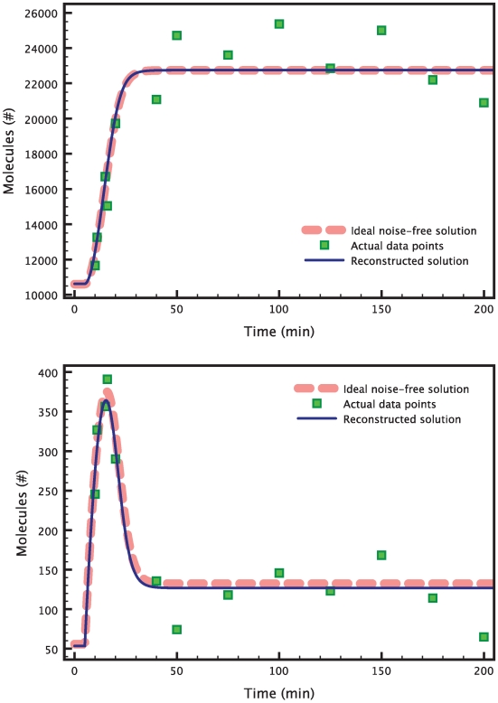
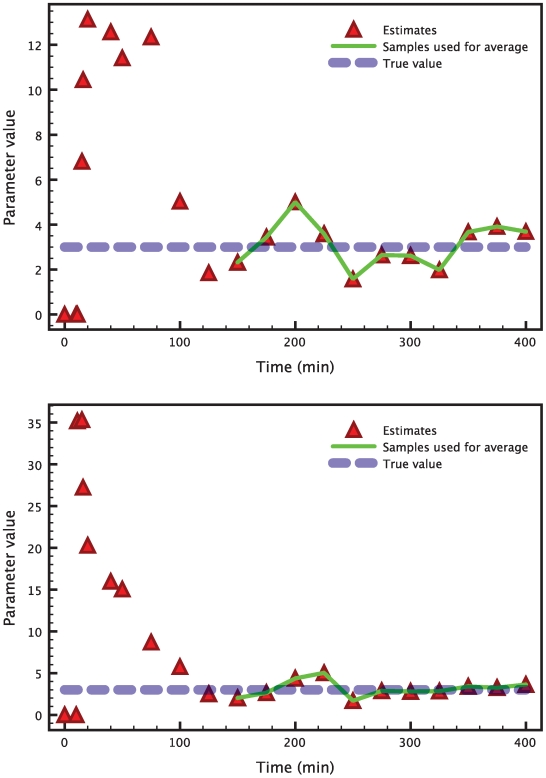
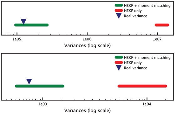
- In the small-parameter heat shock case, the HEKF estimated two parameters whose true value was 3 for both; the text reports the estimation as very accurate despite high noise, and the a posteriori identifiability test at confidence coefficient 0.95 passed for both measurement-noise components.
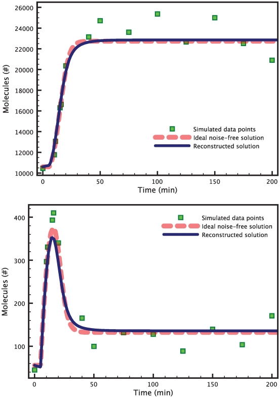
- For the 6-parameter heat shock case, a single HEKF run failed the identifiability test; moment-matching refinement with BFGS found a minimum after 1560 iterations with cost 0.14 in about 3 hours on a MacBook Pro with a single 2.6 GHz processor, and the refined estimates passed the test.
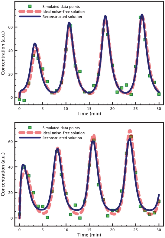
- For the 18-parameter repressilator model, a single HEKF run failed the test; moment-matching refinement with BFGS took 720 iterations (about 26 minutes) and passed all three components, whereas Levenberg-Marquardt least-squares (129 iterations, about 3 minutes) and a genetic algorithm (101 iterations, about 4 minutes) failed.
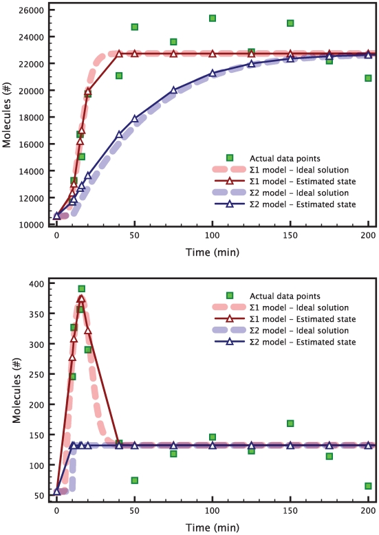
- For model selection in the heat shock example, only model \(M_1\) produced variance interval estimates containing the real measurement-noise variances; model \(M_2\), which lacks the spike in the sigma factor, was rejected as inconsistent with the measurements.
Methods
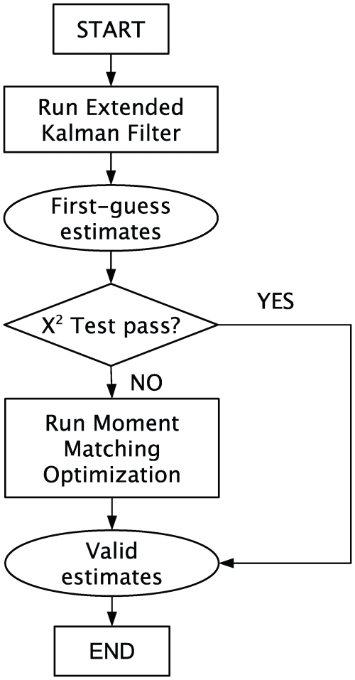
- The model is written as a continuous-time ODE state-space system; parameters are treated as constant states via state extension, and a constrained hybrid extended Kalman filter (HEKF) handles continuous-time dynamics with discrete-time measurements and equality/inequality constraints solved as quadratic programming.
- An a posteriori identifiability test estimates measurement-noise variances from residuals, forms point and interval estimates using the chi-square distribution, and rejects estimates whose intervals do not contain the known real noise variances; if the test fails, a moment-matching optimization minimizes mean and variance mismatch, typically with BFGS.
- Model selection runs the HEKF on candidate models, computes measurement-noise variance estimates for each, discards models whose interval estimates exclude the real variances, and selects the model whose variances match best; examples use simulated noisy data from an E. coli heat shock model (2 and 6 parameters; 22 data points in the small case) and a generalized repressilator model (18 parameters; 30 equally spaced mRNA data points).
Limitations
- The paper states that the extended Kalman filter is not generally optimal for nonlinear systems, may diverge or give biased estimates, can suffer from loss of observability/non-uniqueness after state extension, and is subject to numerical ill-conditioning in covariance propagation; initial estimates too far off can also cause problems.
- The paper states that the process-noise covariance is chosen by the user, the measurement-noise statistics are assumed known, the moment-matching weights are user-selected, and the refinement optimization can be computationally expensive (e.g., about 3 hours for the 6-parameter heat shock case).
- Evident from the text: the demonstrations use in silico simulated measurements rather than real experimental data, and many numerical entries in the tables and some reported percentages are missing from the provided text, limiting independent verification of the exact estimates.
Model-written summary. Check it against the paper before relying on it.
Integrity signals
Registry
Cites
Statistics
Figures
Verification
Claims the paper makes
1 Valid · 1 Not valid · 11 Not checked · 41 Own results and interpretations
Every source the paper cites for this claim was checked and supports it.
In the paper
“These and similar results indicate that the search for the exact individual values of the parameters is a hopeless task in most cases [6].”
§ Parameter Estimation and Model Selection in Computational Biology > Introduction
What the sources say
- Supportedcites [6] M Ashyraliyev, 2008, Parameter estimation and determinability analysis applied to Drosophila gap gene circuits., BMC Systems Biology source
The Background (page unavailable) says that determining all parameters accurately is usually not possible in practice. The Results and Discussion, under Parameter Determinability (page unavailable), further report that no parameter in the analyzed model could be determined individually to the chosen accuracy. Together, these support the citing sentence’s general point without implying that every parameter is indeterminable. (LLM, conf=0.90)
hedged- Asserted: passes — The authors put it forward as true.
- Checkable: passes — It can be checked against evidence.
- Load-bearing: passes — The paper’s conclusions depend on it.
- Based: passes — The paper gives a reason why it holds.
- Supported
A result the paper reports from its own data — it cites no other source for it, so there is none to check. The quote shows it is in the paper.
In the paper
“As in the large parameter space case for the heat shock model, a single run of the HEKF produces estimates that do not satisfy the identifiability test.”
§ Parameter Estimation and Model Selection in Computational Biology > Results > The repressilator
plainstates a causeSingle case- Asserted: passes — The authors put it forward as true.
- Checkable: passes — It can be checked against evidence.
- Load-bearing: passes — The paper’s conclusions depend on it.
- Based: passes — The paper gives a reason why it holds.
A result the paper reports from its own data — it cites no other source for it, so there is none to check. The quote shows it is in the paper.
In the paper
“It is clear that only produces results that are compatible with the measurements.”
§ Parameter Estimation and Model Selection in Computational Biology > Results > A model of the heat shock response in E. coli
boosted- Asserted: passes — The authors put it forward as true.
- Checkable: passes — It can be checked against evidence.
- Load-bearing: passes — The paper’s conclusions depend on it.
- Based: passes — The paper gives a reason why it holds.
A result the paper reports from its own data — it cites no other source for it, so there is none to check. The quote shows it is in the paper.
In the paper
“After a transient, the estimates keep oscillating around the true values of the parameters.”
§ Parameter Estimation and Model Selection in Computational Biology > Results > A model of the heat shock response in E. coli
plainstates an associationSingle case- Asserted: passes — The authors put it forward as true.
- Checkable: passes — It can be checked against evidence.
- Load-bearing: unclear — It is unclear whether the paper’s conclusions depend on it.
- Based: passes — The paper gives a reason why it holds.
A result the paper reports from its own data — it cites no other source for it, so there is none to check. The quote shows it is in the paper.
In the paper
“In this new example, a single run of the HEKF produces values that do not satisfy the identifiability test.”
§ Parameter Estimation and Model Selection in Computational Biology > Results > A model of the heat shock response in E. coli
plainSingle case- Asserted: passes — The authors put it forward as true.
- Checkable: passes — It can be checked against evidence.
- Load-bearing: passes — The paper’s conclusions depend on it.
- Based: passes — The paper gives a reason why it holds.
25 more claims
Create a free account to see all 54 claims and to verify the 12 references still open.
- Probably not a substantial claim. 10
- It may state two separate claims as one. 14
- The quote only partly states this claim. 3
Claims other papers make about this one
Each is checked against this paper’s own text: does it say what the citing paper says it does?
In the citing paper
“The resulting approach may be used for obtaining more accurate estimates of the parameters as well as for model selection.”
From Reverse engineering and identification in systems biology: strategies, perspectives and challenges (2014) · cites this paper as [143]
In the citing paper
“To address the issues of sparse and noisy data, Lillacci & Khammash [143] propose a combination of an extended Kalman filter (a recursive estimator well known in control engineering) with a posteriori identifiability tests and moment-matching optimization.”
From Reverse engineering and identification in systems biology: strategies, perspectives and challenges (2014) · cites this paper as [143]
Self-check
Percentages, sums and reported differences re-computed from the paper’s own numbers.
Each contradiction between two passages listed here was confirmed by an independent check.
Rated minor: it would not touch a result — a value no result rests on, a p-value that stays on the same side of the significance level, or a conflict that is clerical, resolved elsewhere in the paper, or outside its own findings.
In the paper
§ Parameter Estimation and Model Selection in Computational Biology > Results > A model of the heat shock response in E. coli
“we compute the point and interval estimates of the variances of the two components of the measurement noise according to (13) and (15) respectively.”
§ Parameter Estimation and Model Selection in Computational Biology > Methods > An a posteriori identifiability test
“Then, is in the interval(14)with a probability of .”
Citations
Cites
Optimization by Simulated Annealing
Kirkpatrick, S., Gelatt, C. D., & Vecchi, M. P. (1983) · Science · doi:10.1126/science.220.4598.671 · Cited by 45,134 · cited 1×
“Much research has been conducted on the applications to computational biology models of several optimization techniques, such as linear and nonlinear leastsquares fitting [3], simulated annealing [4], genetic algorithms [5], and evolutionary computation [6,7].”
BackgroundProbability, Random Variables, and Stochastic Processes.
Abrahams, J., & Papoulis, A. (1984) · Journal of the American Statistical Association · doi:10.2307/2288754 · Cited by 16,226
Probability, Random Variables, and Stochastic Processes
Miller, I. (1966) · Technometrics · doi:10.1080/00401706.1966.10490365 · Cited by 8,452
Practical Methods of Optimization
Fletcher, R. (2000) · Wiley eBooks · doi:10.1002/9781118723203 · Cited by 7,605
Optimal State Estimation: Kalman, H∞, and Nonlinear Approaches
Simon, D. (2006) · doi:10.1002/0470045345 · Cited by 4,875
A synthetic oscillatory network of transcriptional regulators
Elowitz, M. B., & Leibler, S. (2000) · Nature · doi:10.1038/35002125 · Cited by 4,630 · cited 1×
“The original model of Elowitz and Leibler [39] consists of six equations with four parameters, where all the three genes have the same production and degradation rates, and are affected in the same way by the corresponding repressor.”
BackgroundAnderson, B. D. O., Moore, J. B., & Eslami, M. (1982) · IEEE Transactions on Systems Man and Cybernetics · Cited by 3,195
(2007) · Springer eBooks · doi:10.1007/978-0-387-71107-2 · Cited by 2,687
Srinivas, M., & Patnaik, L. M. (1994) · Computer · doi:10.1109/2.294849 · Cited by 2,180 · cited 1×
“Much research has been conducted on the applications to computational biology models of several optimization techniques, such as linear and nonlinear leastsquares fitting [3], simulated annealing [4], genetic algorithms [5], and evolutionary computation [6,7].”
BackgroundGill, P. E., Murray, W., & Wright, M. H. (2019) · doi:10.1137/1.9781611975604 · Cited by 1,737
Toni, T., Welch, D., Strelkowa, N., Ipsen, A., & Stumpf, M. P. H. (2009) · Journal of The Royal Society Interface · doi:10.1098/rsif.2008.0172 · Cited by 1,498 · cited 3×
“The repressilator is a synthetic gene regulatory network, whose model is frequently used as an example for numerical algorithms [10,27].”
BackgroundMethodUniversally Sloppy Parameter Sensitivities in Systems Biology Models
Gutenkunst, R. N., Waterfall, J. J., Casey, F. P., Brown, K. S., Myers, C. R., & Sethna, J. P. (2007) · PLoS Computational Biology · doi:10.1371/journal.pcbi.0030189 · Cited by 1,261 · cited 1×
“Such ‘‘sloppiness’’ has been suggested as a factor that makes parameter estimation difficult [28].”
BackgroundSimon, D. (2006) · Cited by 1,122
Parameter estimation in biochemical pathways: a comparison of global optimization methods
Moles, C. G., Mendes, P., & Banga, J. R. (2003) · Genome Research · doi:10.1101/gr.1262503 · Cited by 858 · cited 2×
“The latter is suggested as the method of choice for large parameter estimation problems [7].”
BackgroundMethodSequential Monte Carlo without likelihoods
Sisson, S. A., Fan, Y., & Tanaka, M. M. (2007) · Proceedings of the National Academy of Sciences · doi:10.1073/pnas.0607208104 · Cited by 856
It’s a noisy business! Genetic regulation at the nanomolar scale
McAdams, H. H., & Arkin, A. (1999) · Trends in Genetics · doi:10.1016/s0168-9525(98)01659-x · Cited by 848 · cited 1×
“This includes both measurement noise and intrinsic noise, which is well known to play an important role in chemical kinetics when species are present in low copy numbers [9].”
BackgroundMarkov chain Monte Carlo method and its application
Brooks, S. (1998) · Journal of the Royal Statistical Society: Series D (The Statistician) · doi:10.1111/1467-9884.00117 · Cited by 843 · cited 1×
“Nonetheless, the most recent advancements in Bayesian computation, such as Markov chain Monte Carlo techniques [11], ensemble methods [12,13], and sequential Monte Carlo methods that don’t require likelihoods [10,14] have been successfully applied to biological systems, usually in the case of lower-dimensional problem…”
BackgroundMendes, P., & Kell, D. (1998) · Bioinformatics · doi:10.1093/bioinformatics/14.10.869 · Cited by 676 · cited 1×
“Much research has been conducted on the applications to computational biology models of several optimization techniques, such as linear and nonlinear leastsquares fitting [3], simulated annealing [4], genetic algorithms [5], and evolutionary computation [6,7].”
BackgroundColeman, T. F., & Li, Y. (1996) · SIAM Journal on Optimization · doi:10.1137/s1052623494240456 · Cited by 604 · cited 1×
“quadratic programming problem that can be easily solved using standard algorithms, such as reflective Newton methods”
MethodKalman filtering with state equality constraints
Simon, D., & Chia, T. L. (2002) · IEEE Transactions on Aerospace and Electronic Systems · doi:10.1109/7.993234 · Cited by 597 · cited 1×
“To cope with these issues, we apply the constrained estimation technique developed in [30,31].”
MethodState and parameter estimation in chemical and biochemical processes: a tutorial
Dochain, D. (2003) · Journal of Process Control · doi:10.1016/s0959-1524(03)00026-x · Cited by 506 · cited 2×
“State observers can be employed for parameter estimation using the technique of state extension, in which parameters are transformed into states by suitably expanding the system under study [22–24].”
MethodStatistical mechanical approaches to models with many poorly known parameters.
Brown, K. S., & Sethna, J. P. (2003) · Physical Review E · doi:10.1103/physreve.68.021904 · Cited by 398 · cited 2×
“However, it is also known that even if the estimation process is not able to tightly constrain any of the parameter values, the models can still be able to yield significant quantitative predictions [12].”
BackgroundNetwork motifs: Structure does not determine function.
Ingram, P. J., Stumpf, M. P., & Stark, J. (2006) · BMC Genomics · doi:10.1186/1471-2164-7-108 · Cited by 267 · cited 1×
“The knowledge of the parameter values is crucial whenever one wants to obtain quantitative, or even qualitative information from the models [1,2].”
BackgroundAn adaptive high-gain observer for nonlinear systems
Boizot, N., Busvelle, E., & Gauthier, J.-P. (2010) · Automatica · doi:10.1016/j.automatica.2010.06.004 · Cited by 263 · cited 1×
“The controls literature on this subject is vast, but in the context of biological or biochemical systems the classically used approaches include Luenberger-like [17], Kalman filter based, [18–20], and high-gain observers [21].”
MethodBayesian methods in bioinformatics and computational systems biology
Wilkinson, D. J. (2006) · Briefings in Bioinformatics · doi:10.1093/bib/bbm007 · Cited by 230 · cited 1×
“Considerable interested has also been raised by Bayesian methods [8], which can extract information from noisy or”
Plasticity of the cis-Regulatory Input Function of a Gene
Mayo, A. E., Setty, Y., Shavit, S., Zaslaver, A., & Alon, U. (2006) · PLoS Biology · doi:10.1371/journal.pbio.0040045 · Cited by 199 · cited 1×
“The knowledge of the parameter values is crucial whenever one wants to obtain quantitative, or even qualitative information from the models [1,2].”
BackgroundAircraft Turbofan Engine Health Estimation Using Constrained Kalman Filtering
Simon, D., & Simon, D. L. (2005) · Journal of Engineering for Gas Turbines and Power · doi:10.1115/1.1789153 · Cited by 146
Quach, M., Brunel, N., & d'Alché-Buc, F. (2007) · Bioinformatics · doi:10.1093/bioinformatics/btm510 · Cited by 144
Wang, Z., Liu, X., Liu, Y., Liang, J., & Vinciotti, V. (2009) · IEEE Transactions on Computational Biology and Bioinformatics · doi:10.1109/tcbb.2009.5 · Cited by 141
Battogtokh, D., Asch, D. K., Case, M. E., Arnold, J., & Schüttler, H.-B. (2002) · Proceedings of the National Academy of Sciences · doi:10.1073/pnas.262658899 · Cited by 115 · cited 1×
“Nonetheless, the most recent advancements in Bayesian computation, such as Markov chain Monte Carlo techniques [11], ensemble methods [12,13], and sequential Monte Carlo methods that don’t require likelihoods [10,14] have been successfully applied to biological systems, usually in the case of…”
GNU Scientific Library - Reference Manual
Galassi, M. C., Davies, J., Theiler, J. P., Gough, B., Jungman, G., Booth, M., & Fabrice Rossi, A. (2001) · Cited by 102
Sun, X., Jin, L., & Xiong, M. (2008) · PLoS ONE · doi:10.1371/journal.pone.0003758 · Cited by 99 · cited 2×
“We remark that the algorithm we just introduced, as well as the ones employed in other works [25–27], provides unconstrained estimates.”
MethodResultParameter estimation and determinability analysis applied to Drosophila gap gene circuits
Ashyraliyev, M., Jaeger, J., & Blom, J. G. (2008) · BMC Systems Biology · doi:10.1186/1752-0509-2-83 · Cited by 89
An adaptive high-gain observer for nonlinear systems
Bullinger, E., & Allgöwer, F. (2002) · IEEE Conference on Decision and Control (CDC) · doi:10.1109/cdc.1997.649541 · Cited by 67
Advanced Methods and Algorithms for Biological Networks Analysis
El‐Samad, H., Prajna, S., Papachristodoulou, A., Doyle, J. C., & Khammash, M. (2006) · Proceedings of the IEEE · doi:10.1109/jproc.2006.871776 · Cited by 65 · cited 2×
“The following reduced order model of this process has been developed by El-Samad et al. [37].”
BackgroundMethodSelf-citationApplication of modern estimation and identification techniques to chemical processes
Wells, C. H. (1971) · AIChE Journal · doi:10.1002/aic.690170433 · Cited by 48 · cited 1×
“The controls literature on this subject is vast, but in the context of biological or biochemical systems the classically used approaches include Luenberger-like [17], Kalman filter based, [18–20], and high-gain observers [21].”
MethodModel Selection and Mixed-Effects Modeling of HIV Infection Dynamics
Bortz, D. M., & Nelson, P. W. (2006) · Bulletin of Mathematical Biology · doi:10.1007/s11538-006-9084-x · Cited by 48
Hybrid extended Luenberger-asymptotic observer for bioprocess state estimation
Hulhoven, X., Wouwer, A. V., & Bogaerts, P. (2006) · Chemical Engineering Science · doi:10.1016/j.ces.2006.06.018 · Cited by 37
Results Towards Identifiability Properties of Biochemical Reaction Networks
Farina, M., Findeisen, R., Bullinger, E., Bittanti, S., Allgöwer, F., & Wellstead, P. E. (2006) · IEEE Conference on Decision and Control (CDC) · doi:10.1109/cdc.2006.376925 · Cited by 35 · cited 1×
“In control theory, much work has been done in studying this property in terms of another one called observability [23,24].”
BackgroundTests for cycling in a signalling pathway
Müller, T. G., Faller, D., Timmer, J., Swameye, I., Sandra, O., & Klingmüller, U. (2004) · Journal of the Royal Statistical Society Series C: Applied Statistics · doi:10.1111/j.1467-9876.2004.05148.x · Cited by 33 · cited 1×
“Maximum-likelihood estimation [15,16] has also been extensively applied.”
MethodFey, D., Findeisen, R., & Bullinger, E. (2008) · IFAC Proceedings Volumes · doi:10.3182/20080706-5-kr-1001.00053 · Cited by 21 · cited 2×
“State observers can be employed for parameter estimation using the technique of state extension, in which parameters are transformed into states by suitably expanding the system under study [22–24].”
BackgroundMethodHybrid extended Luenberger-asymptotic observer for bioprocess state estimation
Hulhoven, X., Wouwer, A. V., & Bogaerts, P. (2003) · European Control Conference (ECC) · doi:10.23919/ecc.2003.7085347 · Cited by 7 · cited 1×
“The controls literature on this subject is vast, but in the context of biological or biochemical systems the classically used approaches include Luenberger-like [17], Kalman filter based, [18–20], and high-gain observers [21].”
MethodState estimation for a model of gene expression
Lillacci, G., & Valigi, P. (2008) · IEEE International Symposium on Circuits and Systems proceedings · doi:10.1109/iscas.2008.4541850 · Cited by 7 · cited 1×
“The controls literature on this subject is vast, but in the context of biological or biochemical systems the classically used approaches include Luenberger-like [17], Kalman filter based, [18–20], and high-gain observers [21].”
MethodSelf-citationState observers for the estimation of mRNA and protein dynamics
Lillacci, G., & Valigi, P. (2007) · IEEE/NIH Life Science Systems and Applications Workshop · doi:10.1109/lssa.2007.4400896 · Cited by 6 · cited 1×
“This model has been introduced and studied in previous works as part of a deterministic modeling framework for biochemical networks [1, 2].”
MethodSelf-citationFey, D., Findeisen, R., & Bullinger, E. (2008) · ORBi (University of Liège) · Cited by 3
Cited by
Systems biology informed deep learning for inferring parameters and hidden dynamics
Yazdani, A., Lu, L., Raissi, M., & Karniadakis, G. E. (2020) · PLOS Computational Biology · doi:10.1371/journal.pcbi.1007575 · Cited by 329
The Virtual Brain Integrates Computational Modeling and Multimodal Neuroimaging
Ritter, P., Schirner, M., McIntosh, A. R., & Jirsa, V. K. (2013) · Brain Connectivity · doi:10.1089/brain.2012.0120 · Cited by 268
“In the context of biological systems, this problem has been addressed by an approach that combines extended Kalman filtering with a posteriori calculated measures of accuracy of the estimation process based on a v 2 variance test on measurement noise (Lillacci and Khammash, 2010).”
Weak SINDy for partial differential equations
Messenger, D. A., & Bortz, D. M. (2021) · Journal of Computational Physics · doi:10.1016/j.jcp.2021.110525 · Cited by 243
“In the last 20 years, substantial developments have been made at the interface of applied mathematics and statistics to design data-driven model selection algorithms that are both statistically rigorous and computationally efficient (see [4, 11, 12, 21, 23, 24] for both theory and applications).”
BackgroundReverse engineering and identification in systems biology: strategies, perspectives and challenges
Villaverde, A. F., & Banga, J. R. (2014) · Journal of The Royal Society Interface · doi:10.1098/rsif.2013.0505 · Cited by 229
Interval Observers for Time-Varying Discrete-Time Systems
Efimov, D., Perruquetti, W., Raissi, T., & Zolghadri, A. (2013) · IEEE Transactions on Automatic Control · doi:10.1109/tac.2013.2263936 · Cited by 205
Metadata
- Authors
- Lillacci, G., & Khammash, M.
- Affiliations
- University of California, Santa Barbara (US)
- Corresponding author
- Khammash, Mustafa
- Venue
- PLoS Computational Biology
- Publisher
- Public Library of Science (PLoS)
- Published
- 2010-03-05
- Volume
- 6
- Issue
- 3
- Pages
- e1000696
- ISSN
- 1553-734X (ISSN-L)
- 1553-7358
- PMC
- PMC2832681
- OpenAlex
- W2044278781
- Semantic Scholar
- 9a362ed58bcf80e6191bf963bfb5cc5a48f26719
- Cited by
- 325
- References
- 48
- Citations by year
- 2026: 4 · 2025: 13 · 2024: 18 · 2023: 11 · 2022: 16 · 2021: 24 · 2020: 21 · 2019: 29 · 2018: 27 · 2017: 21 · 2016: 19 · 2015: 28 · 2014: 29 · 2013: 34 · 2012: 14
- FWCI
- 8.46
- Type
- journal article
- Language
- en
- Open access
- gold
- doi.org
- Locations
- PLoS Computational Biology (publishedVersion, cc-by)
- PubMed Central (publishedVersion, cc-by)
- PubMed (publishedVersion)
- RePEc: Research Papers in Economics (submittedVersion)
- DOAJ (DOAJ: Directory of Open Access Journals) (submittedVersion, cc-by-sa)
- Figshare (submittedVersion, cc-by)
- Funders
- National Science Foundation (0802008, DAAD19-03-D-0004, 0835847)
- Deutscher Akademischer Austauschdienst
- National Institutes of Health
- National Institute of General Medical Sciences (R01GM049831)
- Division of Electrical, Communications and Cyber Systems (0835847, ECCS-0802008)
- Army Research Office (DAAD 19-03-D-0004, ECCS-0835847)
- Institute for Collaborative Biotechnologies (ECCS-0835847, DAAD19-03-D-0004)
- Topics
- Life Sciences › Biochemistry, Genetics and Molecular Biology › Molecular Biology › Gene Regulatory Network Analysis
- Physical Sciences › Engineering › Control and Systems Engineering › Control Systems and Identification
- Life Sciences › Biochemistry, Genetics and Molecular Biology › Molecular Biology › Microbial Metabolic Engineering and Bioproduction
- Keywords
- parameter estimation, model selection, extended Kalman filter, recursive parameter estimation, identifiability, heat shock response, Escherichia coli, synthetic gene regulation, rate constants, mathematical biology
- MeSH terms
- Algorithms, Animals, Computer Simulation, Gene Expression Regulation, Humans, Models, Biological, Signal Transduction, Proteome, Systems Biology
About these checks
Registry, retraction, Cites and statistics results are computed, not judged, with one exception: a printed reference that no index lists is read once by a model before it counts as a citation error. Claims are extracted by a model and kept only when their quote appears verbatim in the text; each cited source is then checked, with a model’s help, for whether it says what the claim relies on. Those verdicts can be wrong — read the claim’s quote and the cited source before relying on one.
A language model drew the claims from the paper on 2026-10-05, under version 3 of the claim definition (model deepseek-v4.1-flash, prompt extract-v3).
A second model labelled each claim on 2026-10-05 (model jev-1.13-20260917, definition revision gold-guideline-v0.2).
Cited sources are checked with a language model’s help (gpt-6-sol).
Statistics and arithmetic are recomputed, not judged.
Confidence bands are shown only for fields calibrated on our annotated test set. None is calibrated yet, so no band is shown.
What counts as a claim ›How we measure confidence ›How we check this ›
Are you an author, or do you see a problem with this page? Request a review
Data sources
Bibliographic data: Semantic Scholar, OpenAlex, Crossref.
Contains information from the Semantic Scholar Academic Graph Datasets, made available under the ODC Attribution License (ODC-BY 1.0).
Semantic Scholar’s data is described in: Kinney, R., et al. (2023). The Semantic Scholar Open Data Platform. arXiv:2301.10140.
