

The DOI matches its Crossref record; 80 of the 80 references it cites were found in a registry or an index.
Inference of Population Splits and Mixtures from Genome-Wide Allele Frequency Data
Open accessAbstract
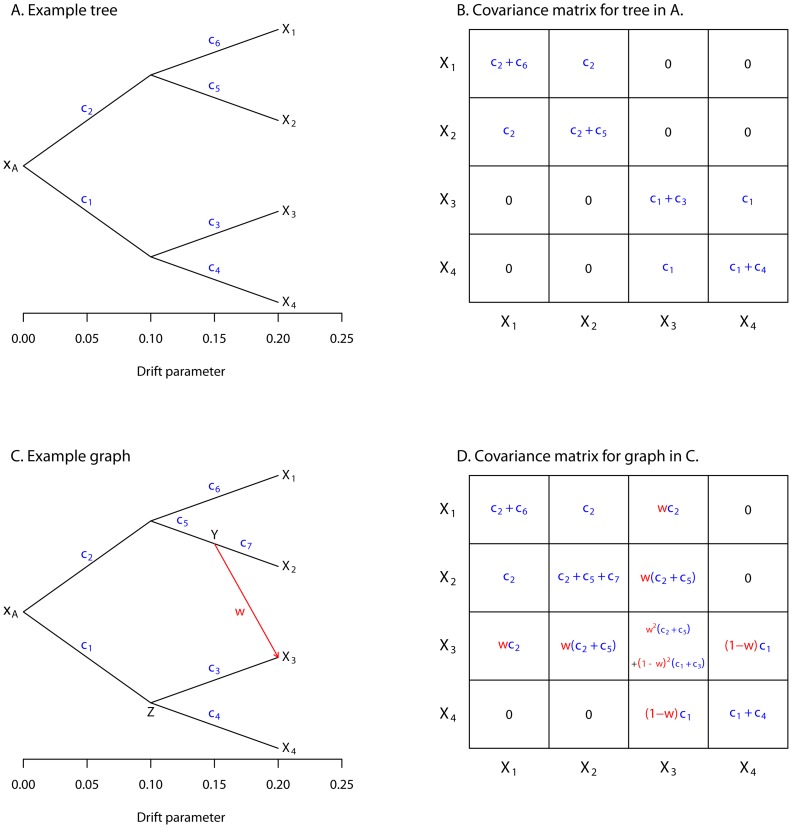
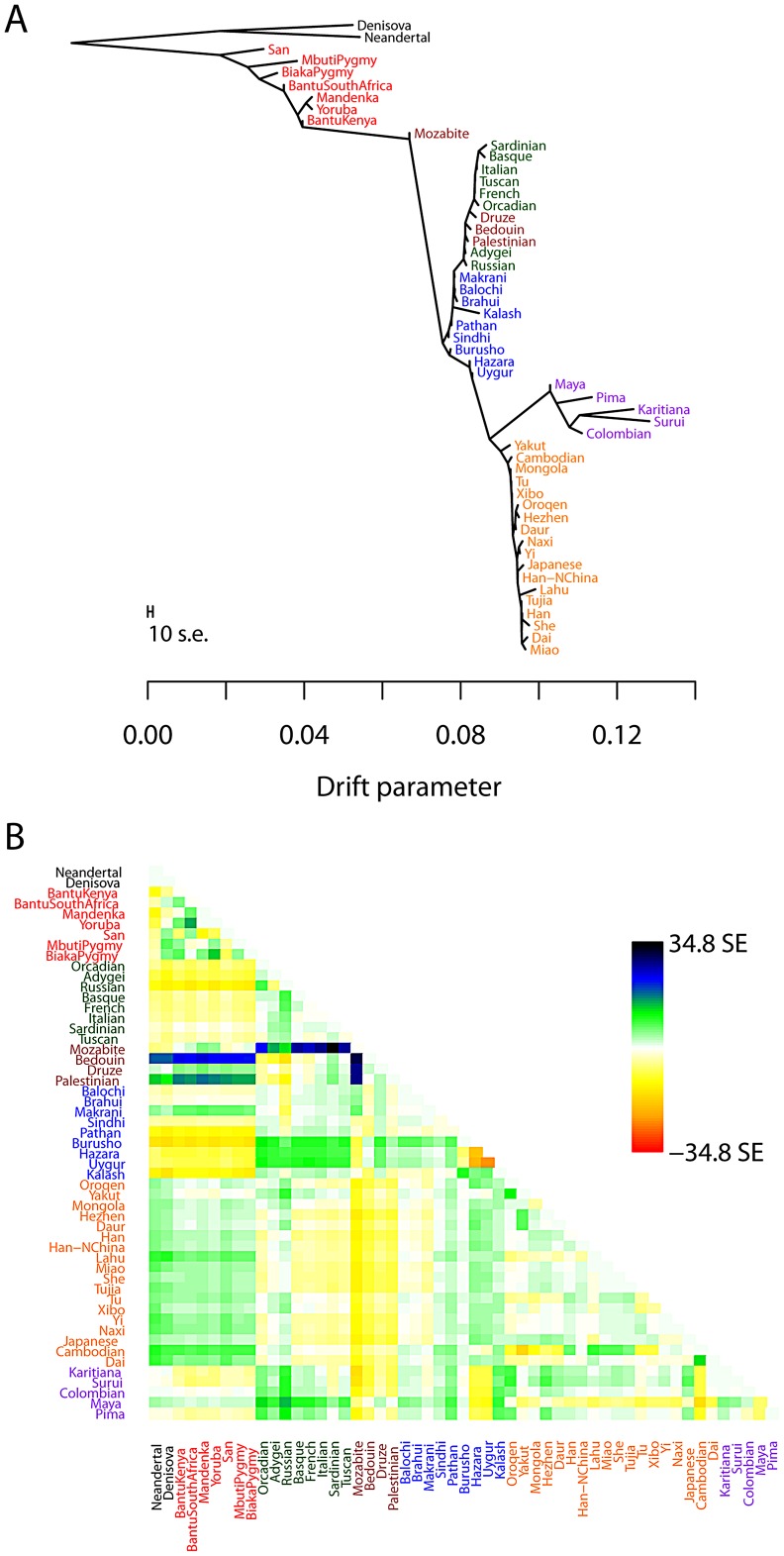
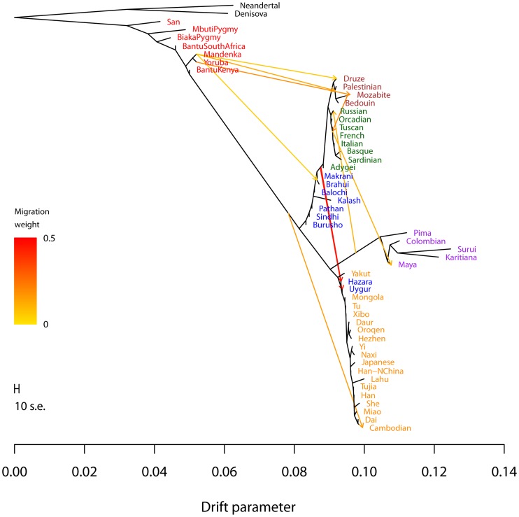
Many aspects of the historical relationships between populations in a species are reflected in genetic data. Inferring these relationships from genetic data, however, remains a challenging task. In this paper, we present a statistical model for inferring the patterns of population splits and mixtures in multiple populations. In our model, the sampled populations in a species are related to their common ancestor through a graph of ancestral populations. Using genome-wide allele frequency data and a Gaussian approximation to genetic drift, we infer the structure of this graph. We applied this method to a set of 55 human populations and a set of 82 dog breeds and wild canids. In both species, we show that a simple bifurcating tree does not fully describe the data; in contrast, we infer many migration events. While some of the migration events that we find have been detected previously, many have not. For example, in the human data, we infer that Cambodians trace approximately 16% of their ancestry to a population ancestral to other extant East Asian populations. In the dog data, we infer that both the boxer and basenji trace a considerable fraction of their ancestry (9% and 25%, respectively) to wolves subsequent to domestication and that East Asian toy breeds (the Shih Tzu and the Pekingese) result from admixture between modern toy breeds and "ancient" Asian breeds. Software implementing the model described here, called TreeMix, is available at http://treemix.googlecode.com.
Overview
The claims and statistics of this paper haven’t been checked yet.
Run the check — free, no account needed. It reads the open-access text and checks the sources it cites.
Integrity signals
Registry
Cites
Statistics
Figures
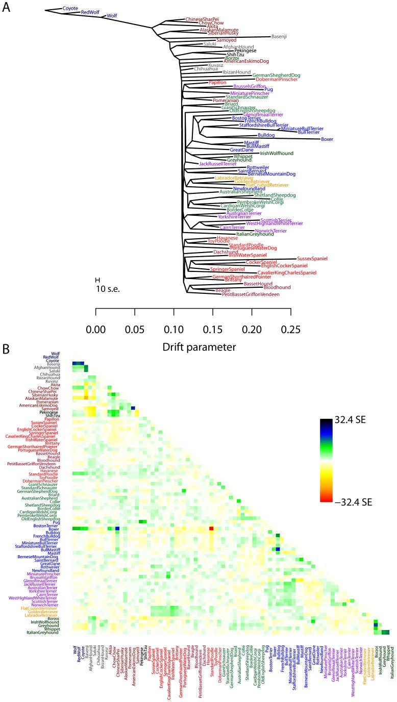
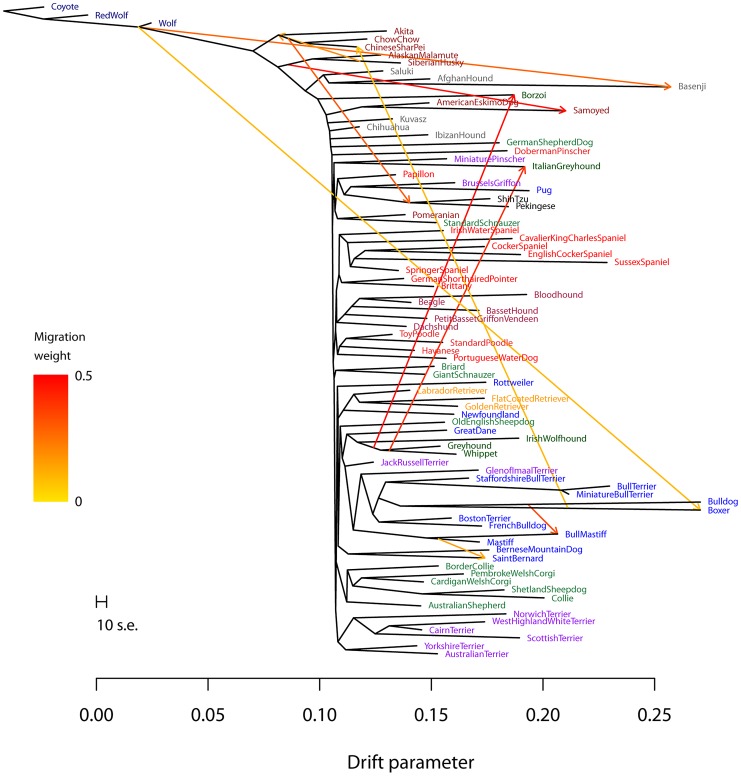
Verification
Claims the paper makes
The claims and statistics of this paper haven’t been checked yet.
Run the check — free, no account needed. It reads the open-access text and checks the sources it cites.
Claims other papers make about this one
Each is checked against this paper’s own text: does it say what the citing paper says it does?
The cited source says what the claim attributes to it.
In the citing paper
“Gene flow from the HGF to domestic HGF in Sudan was indicated in the TreeMix (Pickrell and Pritchard 2012) when m = 1 (supplementary fig. S6, Supplementary Material online) in 99.9% of the bootstrap replicates.”
From Genomic Analyses Unveil Helmeted Guinea Fowl (Numida meleagris) Domestication in West Africa (2021) · cites this paper as Pickrell and Pritchard 2012
Self-check
Percentages, sums and reported differences re-computed from the paper’s own numbers.
The self-check needs the paper’s full text.
Citations
Cites
The neighbor-joining method: a new method for reconstructing phylogenetic trees.
Saitou, N., & Nei, M. (1987) · Molecular Biology and Evolution · doi:10.1093/oxfordjournals.molbev.a040454 · Cited by 59,959
Inference of Population Structure Using Multilocus Genotype Data
Pritchard, J. K., Stephens, M., & Donnelly, P. (2000) · Genetics · doi:10.1093/genetics/155.2.945 · Cited by 33,871
Self-citationESTIMATION OF AVERAGE HETEROZYGOSITY AND GENETIC DISTANCE FROM A SMALL NUMBER OF INDIVIDUALS
Nei, M. (1978) · Genetics · doi:10.1093/genetics/89.3.583 · Cited by 11,368
Application of Phylogenetic Networks in Evolutionary Studies
Huson, D. H., & Bryant, D. (2005) · Molecular Biology and Evolution · doi:10.1093/molbev/msj030 · Cited by 8,895
Solving Least Squares Problems
Lawson, C. L., & Hanson, R. J. (1995) · doi:10.1137/1.9781611971217 · Cited by 7,103
Koller, D., & Friedman, N. (2009) · The MIT Press eBooks · Cited by 6,653
(2009) · Cited by 6,153
Population Structure and Eigenanalysis
Patterson, N., Price, A. L., & Reich, D. (2006) · PLoS Genetics · doi:10.1371/journal.pgen.0020190 · Cited by 5,280
A draft sequence of the Neandertal genome
Green, R. E., Krause, J., Briggs, A. W., Maricic, T., Stenzel, U., Kircher, M., Patterson, N., Li, H., Zhai, W., Fritz, M. H.-Y., et al. (2010) · Science · doi:10.1126/science.1188021 · Cited by 4,318
Mitochondrial DNA and human evolution
Cann, R. L., Stoneking, M., & Wilson, A. C. (1987) · Nature · doi:10.1038/325031a0 · Cited by 3,100
Research works printed but not linked: 1
- N Patterson, 2012, Ancient admixture, Genetics
Cited by
Sorted by citations
Items 1,001–1,008 of 1,008
Posterior predictive checks of coalescent models: P2C2M, an R package
Gruenstaeudl, M., Reid, N. M., Wheeler, G. L., & Carstens, B. C. (2015) · Molecular Ecology Resources · doi:10.1111/1755-0998.12435 · Cited by 23
Owens, G. L., Todesco, M., Bercovich, N., Légaré, J., Mitchell, N., Whitney, K. D., & Rieseberg, L. H. (2021) · Molecular Ecology · doi:10.1111/mec.16008 · Cited by 20
Population genomics of the muskox' resilience in the near absence of genetic variation
Pečnerová, P., Lord, E., Garcia‐Erill, G., Hanghøj, K., Rasmussen, M. S., Meisner, J., Liu, X., van der Valk, T., Santander, C. G., Quinn, L., et al. (2024) · Molecular Ecology · doi:10.1111/mec.17205 · Cited by 19
Lins, L. S. F., Trojahn, S., Sockell, A., Yee, M.-C., Tatarenkov, A., Bustamante, C. D., Earley, R. L., & Kelley, J. L. (2018) · Genome · doi:10.1139/gen-2017-0188 · Cited by 18
BioMaster: Multi-agent System for Automated Bioinformatics Analysis Workflow
Su, H., Long, W., & Zhang, Y. (2025) · doi:10.1101/2025.01.23.634608 · Cited by 18
Genomic analyses overturn two long-standing homoploid hybrid speciation hypotheses
Goulet‐Scott, B. E., Garner, A. G., & Hopkins, R. (2021) · Evolution · doi:10.1111/evo.14279 · Cited by 14
Genomic Analyses Unveil Helmeted Guinea Fowl (Numida meleagris) Domestication in West Africa
Shen, Q.-K., Peng, M.-S., Adeola, A. C., Kui, L., Duan, S., Miao, Y.-W., Eltayeb, N. M., Lichoti, J. K., Otecko, N. O., Strillacci, M. G., et al. (2021) · Genome Biology and Evolution · doi:10.1093/gbe/evab090 · Cited by 15
Moreno-Mayar, J. V. (2022) · G3 Genes|Genomes|Genetics · doi:10.1093/g3journal/jkab357 · Cited by 4
Metadata
- Authors
- Pickrell, J. K., & Pritchard, J. K.
- Affiliations
- University of Chicago (US)
- Howard Hughes Medical Institute (US)
- Corresponding author
- Pickrell, Joseph K.
- Pritchard, Jonathan K.
- Venue
- PLoS Genetics
- Publisher
- Public Library of Science (PLoS)
- Published
- 2012-11-15
- Volume
- 8
- Issue
- 11
- Pages
- e1002967
- ISSN
- 1553-7390 (ISSN-L)
- 1553-7404
- PMC
- PMC3499260
- OpenAlex
- W2093044565
- Cited by
- 2,731
- References
- 79
- Citations by year
- 2026: 223 · 2025: 260 · 2024: 362 · 2023: 271 · 2022: 277 · 2021: 346 · 2020: 222 · 2019: 175 · 2018: 180 · 2017: 117 · 2016: 120 · 2015: 80 · 2014: 65 · 2013: 22 · 2012: 7
- FWCI
- 33.43
- Type
- journal article
- Language
- en
- Open access
- gold
- doi.org
- Locations
- PLoS Genetics (publishedVersion, cc-by)
- Europe PMC (PubMed Central) (publishedVersion, cc-by)
- PubMed Central (publishedVersion, cc-by)
- PubMed (publishedVersion)
- arXiv (Cornell University) (submittedVersion)
- Figshare (submittedVersion, cc-by)
- Knowledge@UChicago (University of Chicago) (submittedVersion, cc-by-nc-nd)
- RePEc: Research Papers in Economics (submittedVersion)
- DOAJ (DOAJ: Directory of Open Access Journals) (submittedVersion, cc-by-sa)
- Nature Precedings (submittedVersion)
- arXiv (Cornell University)
- University of Chicago (cc-by)
- Funders
- Howard Hughes Medical Institute
- National Institutes of Health
- National Institute of Mental Health (R01MH084703, MH084703)
- National Institute of General Medical Sciences (F32GM103098)
- Topics
- Life Sciences › Biochemistry, Genetics and Molecular Biology › Genetics › Forensic and Genetic Research
- Life Sciences › Biochemistry, Genetics and Molecular Biology › Genetics › Genetic diversity and population structure
- Life Sciences › Biochemistry, Genetics and Molecular Biology › Genetics › Genetic Associations and Epidemiology
- Keywords
- population admixture, population structure inference, migration events, dog breeds, wild canids, genetic drift, TreeMix, dog domestication, Shih Tzu, Pekingese
- MeSH terms
- Algorithms, Animals, Breeding, Dogs, Gene Frequency, Humans, Models, Genetic, Population, Wolves, Polymorphism, Single Nucleotide, Genetic Drift, Genome-Wide Association Study
About these checks
Registry, retraction, Cites and statistics results are computed, not judged, with one exception: a printed reference that no index lists is read once by a model before it counts as a citation error. Claims are extracted by a model and kept only when their quote appears verbatim in the text; each cited source is then checked, with a model’s help, for whether it says what the claim relies on. Those verdicts can be wrong — read the claim’s quote and the cited source before relying on one.
Statistics and arithmetic are recomputed, not judged.
Confidence bands are shown only for fields calibrated on our annotated test set. None is calibrated yet, so no band is shown.
What counts as a claim ›How we measure confidence ›How we check this ›
Are you an author, or do you see a problem with this page? Request a review
