

The DOI matches its Crossref record; 74 of the 74 references it cites were found in a registry or an index.
Inferring Population Size History from Large Samples of Genome-Wide Molecular Data - An Approximate Bayesian Computation Approach
Open accessPublished version of a preprint
Abstract
Inferring the ancestral dynamics of effective population size is a long-standing question in population genetics, which can now be tackled much more accurately thanks to the massive genomic data available in many species. Several promising methods that take advantage of whole-genome sequences have been recently developed in this context. However, they can only be applied to rather small samples, which limits their ability to estimate recent population size history. Besides, they can be very sensitive to sequencing or phasing errors. Here we introduce a new approximate Bayesian computation approach named PopSizeABC that allows estimating the evolution of the effective population size through time, using a large sample of complete genomes. This sample is summarized using the folded allele frequency spectrum and the average zygotic linkage disequilibrium at different bins of physical distance, two classes of statistics that are widely used in population genetics and can be easily computed from unphased and unpolarized SNP data. Our approach provides accurate estimations of past population sizes, from the very first generations before present back to the expected time to the most recent common ancestor of the sample, as shown by simulations under a wide range of demographic scenarios. When applied to samples of 15 or 25 complete genomes in four cattle breeds (Angus, Fleckvieh, Holstein and Jersey), PopSizeABC revealed a series of population declines, related to historical events such as domestication or modern breed creation. We further highlight that our approach is robust to sequencing errors, provided summary statistics are computed from SNPs with common alleles.
Overview
The claims and statistics of this paper haven’t been checked yet.
Run the check — free, no account needed. It reads the open-access text and checks the sources it cites.
Integrity signals
Registry
Cites
Statistics
Figures
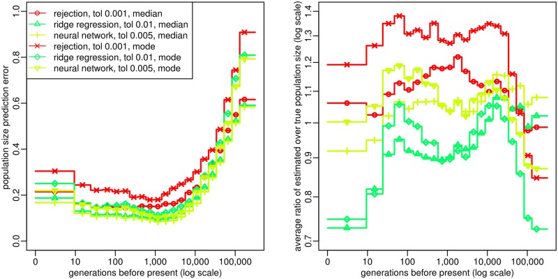
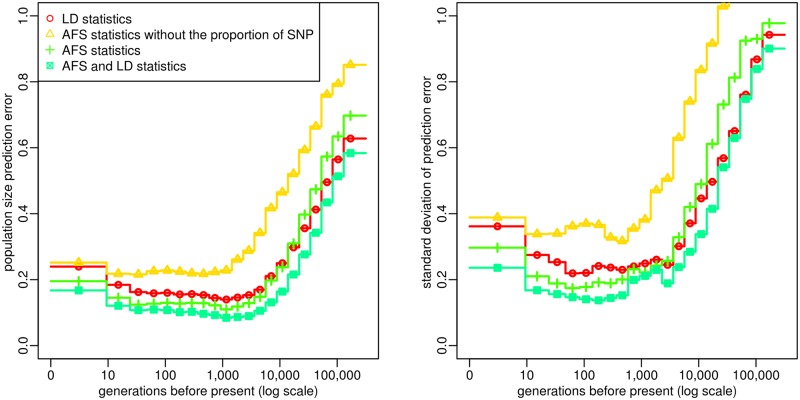
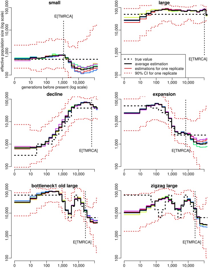
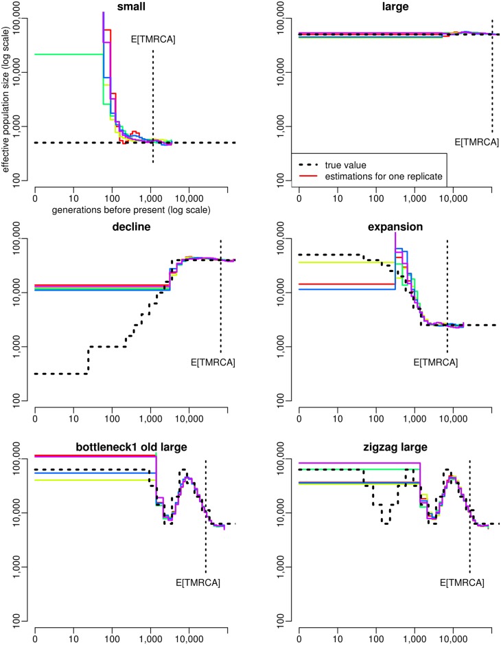
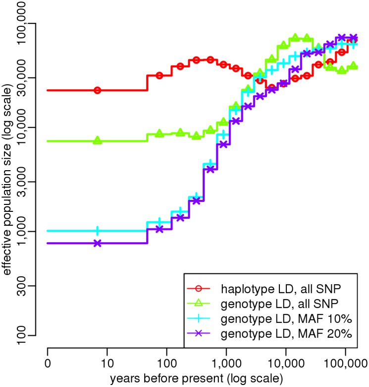
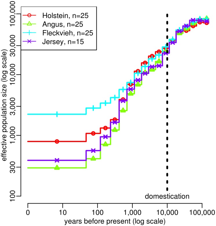
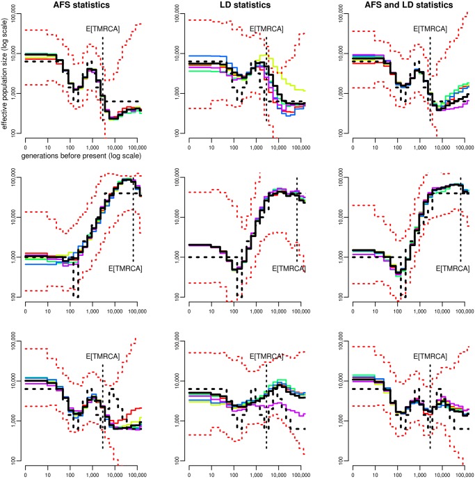
Verification
Claims the paper makes
The claims and statistics of this paper haven’t been checked yet.
Run the check — free, no account needed. It reads the open-access text and checks the sources it cites.
Claims other papers make about this one
Each is checked against this paper’s own text: does it say what the citing paper says it does?
The source backs part of the claim, not all of it — or backs it for a different population, condition or comparison.
In the citing paper
“This pattern was also observed in the analysis of PopSizeABC (Boitard et al. 2016) (supplementary fig. S8, Supplementary Material online).”
From Genomic Analyses Unveil Helmeted Guinea Fowl (Numida meleagris) Domestication in West Africa (2021) · cites this paper as Boitard et al. 2016
Experimental — accuracy not yet measured
Self-check
Percentages, sums and reported differences re-computed from the paper’s own numbers.
The self-check needs the paper’s full text.
Citations
Cites
GCTA: a tool for genome-wide complex trait analysis
Yang, J., Lee, S. H., Goddard, M. E., & Visscher, P. M. (2011) · The American Journal of Human Genetics · doi:10.1016/j.ajhg.2010.11.011 · Cited by 8,279
Approximate Bayesian computation in population genetics
Beaumont, M. A., Zhang, W., & Balding, D. J. (2002) · Genetics · doi:10.1093/genetics/162.4.2025 · Cited by 2,932
Inference of human population history from individual whole-genome sequences
Li, H., & Durbin, R. (2011) · Nature · doi:10.1038/nature10231 · Cited by 2,590
Generating samples under a Wright–Fisher neutral model of genetic variation
Hudson, R. R. (2002) · Bioinformatics · doi:10.1093/bioinformatics/18.2.337 · Cited by 2,397
Gutenkunst, R. N., Hernandez, R. D., Williamson, S. H., & Bustamante, C. D. (2009) · PLoS Genetics · doi:10.1371/journal.pgen.1000695 · Cited by 1,906
Robust Demographic Inference from Genomic and SNP Data
Excoffier, L., Dupanloup, I., Huerta‐Sánchez, E., Sousa, V. C., & Foll, M. (2013) · PLoS Genetics · doi:10.1371/journal.pgen.1003905 · Cited by 1,480
Analyses of pig genomes provide insight into porcine demography and evolution
Groenen, M. A. M., Archibald, A. L., Uenishi, H., Tuggle, C. K., Takeuchi, Y., Rothschild, M. F., Rogel-Gaillard, C., Park, C., Milan, D., Megens, H., et al. (2012) · Nature · doi:10.1038/nature11622 · Cited by 1,424
Approximate Bayesian Computation (ABC) in practice
Csilléry, K., Blum, M. G. B., Gaggiotti, O. E., & François, O. (2010) · Trends in Ecology & Evolution · doi:10.1016/j.tree.2010.04.001 · Cited by 1,302
Domestication and early agriculture in the Mediterranean Basin: Origins, diffusion, and impact
Zeder, M. A. (2008) · Proceedings of the National Academy of Sciences · doi:10.1073/pnas.0801317105 · Cited by 1,160
Inferring human population size and separation history from multiple genome sequences
Schiffels, S., & Durbin, R. (2014) · Nature Genetics · doi:10.1038/ng.3015 · Cited by 1,073
Kijas, J., Lenstra, J. A., Hayes, B. J., Boitard, S., Porto-Neto, L. R., Cristobal, M. S., Servin, B., McCulloch, R. J., Whan, V., Gietzen, K., et al. (2012) · PLoS Biology · doi:10.1371/journal.pbio.1001258 · Cited by 936
Self-citationInterrogating a high-density SNP map for signatures of natural selection.Preprint
Akey, J., Zhang, G., Zhang, K., Jin, L., & Shriver, M. (2002) · Genome Research · doi:10.1101/gr.631202 · Cited by 932
Whole-genome sequencing of 234 bulls facilitates mapping of monogenic and complex traits in cattle
Daetwyler, H. D., Capitan, A., Pausch, H., Stothard, P., van Binsbergen, R., Brøndum, R. F., Liao, X., Djari, A., Rodriguez, S., Grohs, C., et al. (2014) · Nature Genetics · doi:10.1038/ng.3034 · Cited by 868
Genome-wide survey of SNP variation uncovers the genetic structure of cattle breeds
The Bovine HapMap Consortium, Gibbs, R. A., Taylor, J. F., Van Tassell, C. P., Barendse, W., Eversole, K. A., Gill, C. A., Green, R. D., Hamernik, D. L., Kappes, S. M., et al. (2009) · Science · doi:10.1126/science.1167936 · Cited by 868
Estimation of effective population size from data on linkage disequilibrium
Hill, W. G. (1981) · Genetics Research · doi:10.1017/s0016672300020553 · Cited by 861
Properties of a neutral allele model with intragenic recombination
Hudson, R. R. (1983) · Theoretical Population Biology · doi:10.1016/0040-5809(83)90013-8 · Cited by 816
abc: an R package for approximate Bayesian computation (ABC)
Csilléry, K., François, O., & Blum, M. G. B. (2012) · Methods in Ecology and Evolution · doi:10.1111/j.2041-210x.2011.00179.x · Cited by 709
Cornuet, J., Santos, F., Beaumont, M., Robert, C. P., Marin, J., Balding, D. J., Guillemaud, T., & Estoup, A. (2008) · Bioinformatics · doi:10.1093/bioinformatics/btn514 · Cited by 690
Species-specific responses of Late Quaternary megafauna to climate and humans
Lorenzen, E. D., Nogués-Bravo, D., Orlando, L., Weinstock, J., Binladen, J., Marske, K. A., Ugan, A., Borregaard, M. K., Gilbert, M. T. P., Nielsen, R., et al. (2011) · Nature · doi:10.1038/nature10574 · Cited by 638
A General Approach for Haplotype Phasing across the Full Spectrum of Relatedness
O'Connell, J., Gurdasani, D., Delaneau, O., Pirastu, N., Ulivi, S., Cocca, M., Traglia, M., Huang, J., Huffman, J. E., Rudan, I., et al. (2014) · PLoS Genetics · doi:10.1371/journal.pgen.1004234 · Cited by 593
Exploring population size changes using SNP frequency spectra
Liu, X., & Fu, Y. (2015) · Nature Genetics · doi:10.1038/ng.3254 · Cited by 481
Skyline‐plot methods for estimating demographic history from nucleotide sequences
Ho, S. Y. W., & Shapiro, B. (2011) · Molecular Ecology Resources · doi:10.1111/j.1755-0998.2011.02988.x · Cited by 481
Novel Multilocus Measure of Linkage Disequilibrium to Estimate Past Effective Population SizePreprint
Hayes, B. J., Visscher, P. M., McPartlan, H. C., & Goddard, M. E. (2003) · Genome Research · doi:10.1101/gr.387103 · Cited by 456
Non-linear regression models for Approximate Bayesian Computation
Blum, M. G. B., & François, O. (2009) · Statistics and Computing · doi:10.1007/s11222-009-9116-0 · Cited by 449
An Integrated Framework for the Inference of Viral Population History From Reconstructed Genealogies
Pybus, O. G., Rambaut, A., & Harvey, P. (2000) · Genetics · doi:10.1093/genetics/155.3.1429 · Cited by 446
Nielsen, R., Korneliussen, T., Albrechtsen, A., Li, Y., & Wang, J. (2012) · PLoS ONE · doi:10.1371/journal.pone.0037558 · Cited by 424 · cited 1×
“Such algorithms are available both for AFS [55] and LD statistics [56], which is another advantage of using these standard summary statistics.”
MethodThree crocodilian genomes reveal ancestral patterns of evolution among archosaurs
Green, R. E., Braun, E. L., Armstrong, J., Earl, D., Nguyen, N., Hickey, G., Vandewege, M. W., St. John, J. A., Capella-Gutiérrez, S., Castoe, T. A., et al. (2014) · Science · doi:10.1126/science.1254449 · Cited by 359
A Comparative Review of Dimension Reduction Methods in Approximate Bayesian Computation
Blum, M. G. B., Nunes, M. A., Prangle, D., & Sisson, S. A. (2013) · Statistical Science · doi:10.1214/12-sts406 · Cited by 355
Approximating the coalescent with recombination
McVean, G., & Cardin, N. J. (2005) · Philosophical Transactions of the Royal Society B Biological Sciences · doi:10.1098/rstb.2005.1673 · Cited by 354
Zhao, S., Zheng, P., Dong, S., Zhan, X., Wu, Q., Guo, X., Hu, Y., He, W., Zhang, S., Fan, W., et al. (2012) · Nature Genetics · doi:10.1038/ng.2494 · Cited by 353
Heller, R., Chikhi, L., & SIEGISMUND, H. R. (2013) · PLoS ONE · doi:10.1371/journal.pone.0062992 · Cited by 352
Mazet, O., Rodríguez, W., Grusea, S., Boitard, S., & Chikhi, L. (2015) · Heredity · doi:10.1038/hdy.2015.104 · Cited by 338
Self-citationChikhi, L., Sousa, V. C., Luisi, P., Goossens, B., & Beaumont, M. (2010) · Genetics · doi:10.1534/genetics.110.118661 · Cited by 309
Leroy, G., Mary‐Huard, T., Verrier, É., Danvy, S., Charvolin-Lemaire, E., & Danchin-Burge, C. (2013) · Genetics Selection Evolution · doi:10.1186/1297-9686-45-1 · Cited by 260
Inbreeding in Danish Dairy Cattle Breeds
Sørensen, A. C., Sørensen, M. K., & Berg, P. (2005) · Journal of Dairy Science · doi:10.3168/jds.s0022-0302(05)72861-7 · Cited by 236
Inferring Demographic History from a Spectrum of Shared Haplotype Lengths
Harris, K., & Nielsen, R. (2013) · PLoS Genetics · doi:10.1371/journal.pgen.1003521 · Cited by 230
Marjoram, P., & Wall, J. D. (2006) · BMC Genetics · doi:10.1186/1471-2156-7-16 · Cited by 221
Demographic History of Oceania Inferred from Genome-wide Data
Wollstein, A., Lao, O., Becker, C., Brauer, S., Trent, R. J., Nürnberg, P., Stoneking, M., & Kayser, M. (2010) · Current Biology · doi:10.1016/j.cub.2010.10.040 · Cited by 218
Insights into the Genetic History of French Cattle from Dense SNP Data on 47 Worldwide Breeds
Gautier, M., Laloë, D., & Moazami‐Goudarzi, K. (2010) · PLoS ONE · doi:10.1371/journal.pone.0013038 · Cited by 214
Lectures on Probability Theory and Statistics
Barlow, M. T., & Nualart, D. (1998) · Lecture notes in mathematics · doi:10.1007/bfb0092536 · Cited by 201
Sheehan, S., Harris, K., & Song, Y. S. (2013) · Genetics · doi:10.1534/genetics.112.149096 · Cited by 187
Drastic population fluctuations explain the rapid extinction of the passenger pigeon
Hung, C.-M., Shaner, P.-J. L., Zink, R. M., Liu, W.-C., Chu, T.-C., Huang, W.-S., & Li, S.-H. (2014) · Proceedings of the National Academy of Sciences · doi:10.1073/pnas.1401526111 · Cited by 186
On the History of Cattle Genetic Resources
Felius, M., Beerling, M.-L., Buchanan, D., Theunissen, B., Koolmees, P., & Lenstra, J. (2014) · Diversity · doi:10.3390/d6040705 · Cited by 176
Estimation of historical effective population size using linkage disequilibria with marker data
Corbin, L. J., LIU, A. Y. H., Bishop, S. C., & Woolliams, J. A. (2012) · Journal of Animal Breeding and Genetics · doi:10.1111/j.1439-0388.2012.01003.x · Cited by 161
McEvoy, B. P., Powell, J. E., Goddard, M. E., & Visscher, P. M. (2011) · Genome Research · doi:10.1101/gr.119636.110 · Cited by 161
Genetic Variants in REC8, RNF212, and PRDM9 Influence Male Recombination in Cattle
Sandor, C., Li, W., Coppieters, W. R., Druet, T., Charlier, C., & Georges, M. (2012) · PLoS Genetics · doi:10.1371/journal.pgen.1002854 · Cited by 151
H UMAN M IGRATIONS AND P OPULATION S TRUCTURE : What We Know and Why it Matters
Goldstein, D. B., & Chikhi, L. (2002) · Annual Review of Genomics and Human Genetics · doi:10.1146/annurev.genom.3.022502.103200 · Cited by 138
High-density marker imputation accuracy in sixteen French cattle breeds
Hozé, C., Fouilloux, M.-N. M.-N., Venot, É., Guillaume, F., Dassonneville, R., Fritz, S., Ducrocq, V., Phocas, F., Boichard, D., & Croiseau, P. (2013) · Genetics Selection Evolution · doi:10.1186/1297-9686-45-33 · Cited by 134
MacLeod, I. M., Larkin, D. M., Lewin, H. A., Hayes, B. J., & Goddard, M. E. (2013) · Molecular Biology and Evolution · doi:10.1093/molbev/mst125 · Cited by 133
Patin, É., Siddle, K. J., Laval, G., Quach, H., Harmant, C., Becker, N. S., Froment, A., Regnault, B., Lemée, L., Gravel, S., et al. (2014) · Nature Communications · doi:10.1038/ncomms4163 · Cited by 130
Nadachowska‐Brzyska, K., Burri, R., Olason, P. I., Kawakami, T., Smeds, L., & Ellegren, H. (2013) · PLoS Genetics · doi:10.1371/journal.pgen.1003942 · Cited by 127
Inferring population size changes with sequence and SNP data: lessons from human bottlenecks
Gattepaille, L. M., Jakobsson, M., & Blum, M. G. B. (2013) · Heredity · doi:10.1038/hdy.2012.120 · Cited by 125
Peter, B. M., Wegmann, D., & Excoffier, L. (2010) · Molecular Ecology · doi:10.1111/j.1365-294x.2010.04783.x · Cited by 124
On the Breeds of Cattle—Historic and Current Classifications
Felius, M., Koolmees, P. A., Theunissen, B., & Lenstra, J. A. (2011) · Diversity · doi:10.3390/d3040660 · Cited by 102
Quéméré, E., Amelot, X., Pierson, J., Crouau‐Roy, B., & Chikhi, L. (2012) · Proceedings of the National Academy of Sciences · doi:10.1073/pnas.1200153109 · Cited by 100
Mazet, O., Rodríguez, W., & Chikhi, L. (2015) · Theoretical Population Biology · doi:10.1016/j.tpb.2015.06.003 · Cited by 97
Self-citationLinkage Disequilibrium Between Loci With Unknown Phase
Rogers, A. R., & Huff, C. D. (2009) · Genetics · doi:10.1534/genetics.108.093153 · Cited by 94
Edwards, C. J., Ginja, C., Kantanen, J., Pérez-Pardal, L., Tresset, A., Stock, F., Gama, L. T., Penedo, M. C. T., Bradley, D. G., Lenstra, J. A., et al. (2011) · PLoS ONE · doi:10.1371/journal.pone.0015922 · Cited by 88
Effective population size of an indigenous Swiss cattle breed estimated from linkage disequilibrium
Flury, C., Tapio, M., Sonstegard, T. S., Drögemüller, C., Leeb, T., Simianer, H., Hanotte, O., & Rieder, S. (2010) · Journal of Animal Breeding and Genetics · doi:10.1111/j.1439-0388.2010.00862.x · Cited by 86
Detecting past changes of effective population size
Nikolic, N., & Chevalet, C. (2014) · Evolutionary Applications · doi:10.1111/eva.12170 · Cited by 81
Bhaskar, A., Wang, Y. X. R., & Song, Y. S. (2015) · Genome Research · doi:10.1101/gr.178756.114 · Cited by 77
Bhaskar, A., & Song, Y. S. (2014) · The Annals of Statistics · doi:10.1214/14-aos1264 · Cited by 75
Lukić, S., & Hey, J. (2012) · Genetics · doi:10.1534/genetics.112.141846 · Cited by 65
Inferring Bottlenecks from Genome-Wide Samples of Short Sequence Blocks
Bunnefeld, L., Frantz, L., & Lohse, K. (2015) · Genetics · doi:10.1534/genetics.115.179861 · Cited by 62
How Population Growth Affects Linkage Disequilibrium
Rogers, A. R. (2014) · Genetics · doi:10.1534/genetics.114.166454 · Cited by 61
Veeramah, K. R., Woerner, A. E., Johnstone, L. M., Gut, I. G., Gut, M. O., Marquès‐Bonet, T., Carbone, L., Wall, J. D., & Hammer, M. F. (2015) · Genetics · doi:10.1534/genetics.115.174425 · Cited by 55
Lectures on Probability Theory and Statistics
Albeverio, S. A., Schachermayer, W., Talagrand, M., Bernard, P., & Saint-Flour, E. D. D. P. 1. (2003) · Lecture notes in mathematics · doi:10.1007/3-540-44922-1 · Cited by 52
Li, S., & Jakobsson, M. (2012) · BMC Genetics · doi:10.1186/1471-2156-13-22 · Cited by 45
Recent population decline and selection shape diversity of taxol‐related genes
Burgarella, C., Navascués, M., Zabal‐Aguirre, M., Berganzo, E., Riba, M., Mayol, M., Vendramin, G. G., & González‐Martínez, S. C. (2012) · Molecular Ecology · doi:10.1111/j.1365-294x.2012.05532.x · Cited by 34
Shin, D., Cho, K., Park, K.-D., Lee, H. J., & Kim, H. (2013) · Asian-Australasian Journal of Animal Sciences · doi:10.5713/ajas.2013.13320 · Cited by 31
Maruki, T., & Lynch, M. (2014) · Genetics · doi:10.1534/genetics.114.165514 · Cited by 27
Inferring the History of Population Size Change from Genome-Wide SNP Data
Theunert, C., Tang, K., Lachmann, M., Hu, S., & Stoneking, M. (2012) · Molecular Biology and Evolution · doi:10.1093/molbev/mss175 · Cited by 23
Analyse généalogique des races bovines laitières françaises
Boichard, D., Maignel, L., & Verrier, É. (2016) · INRAE Productions Animales · doi:10.20870/productions-animales.1996.9.5.4071 · Cited by 21
Bhaskar, A., Wang, Y. X. R., & Song, Y. S. (2014) · bioRxiv (Cold Spring Harbor Laboratory) · doi:10.1101/006742 · Cited by 5
Cited by
Sorted by citations
Hayes, B. J., & Daetwyler, H. D. (2018) · Annual Review of Animal Biosciences · doi:10.1146/annurev-animal-020518-115024 · Cited by 476
Stairway Plot 2: demographic history inference with folded SNP frequency spectra
Liu, X., & Fu, Y. (2020) · Genome biology · doi:10.1186/s13059-020-02196-9 · Cited by 492
Fuentes‐Pardo, A. P., & Ruzzante, D. E. (2017) · Molecular Ecology · doi:10.1111/mec.14264 · Cited by 417
Genomics advances the study of inbreeding depression in the wild
Kardos, M. D., Taylor, H. R., Ellegren, H., Luikart, G., & Allendorf, F. W. (2016) · Evolutionary Applications · doi:10.1111/eva.12414 · Cited by 405
The Genome Landscape of Indigenous African Cattle
Kim, J., Hanotte, O., Mwai, O. A., Dessie, T., Bashir, S., Diallo, B., Agaba, M., Kim, K., Kwak, W., Sung, S., et al. (2017) · Genome biology · doi:10.1186/s13059-017-1153-y · Cited by 271
Metadata
- Authors
- Boitard, S., Rodríguez, W., Jay, F., Mona, S., & Austerlitz, F.
- Affiliations
- Centre National de la Recherche Scientifique (FR)
- Université Paris-Sud (FR)
- Venue
- PLoS Genetics
- Publisher
- Public Library of Science (PLoS)
- Published
- 2016-03-04
- Volume
- 12
- Issue
- 3
- Pages
- e1005877
- ISSN
- 1553-7390 (ISSN-L)
- 1553-7404
- PMC
- PMC4778914
- OpenAlex
- W2292463482
- Cited by
- 190
- References
- 73
- Citations by year
- 2026: 16 · 2025: 13 · 2024: 30 · 2023: 22 · 2022: 13 · 2021: 23 · 2020: 15 · 2019: 11 · 2018: 25 · 2017: 17 · 2016: 5
- FWCI
- 15.60
- Type
- journal article
- Language
- en
- Open access
- gold
- doi.org
- Licence
- Locations
- PLoS Genetics (publishedVersion, cc-by)
- bioRxiv (Cold Spring Harbor Laboratory) (acceptedVersion, cc-by-nc)
- Europe PMC (PubMed Central) (publishedVersion, cc-by)
- PubMed Central (publishedVersion, cc-by)
- PubMed (publishedVersion)
- HAL (submittedVersion, cc-by)
- HAL (submittedVersion, other-oa)
- DOAJ (DOAJ: Directory of Open Access Journals) (submittedVersion, cc-by-sa)
- Figshare (submittedVersion, cc-by)
- Funders
- Indian National Science Academy
- Agence Nationale de la Recherche (ANR-10-GENM-0014, ANR-12, ANR-10, ANR-12-BSV7-0012)
- Université de Toulouse
- Centre National de la Recherche Scientifique
- Institut National de la Recherche Agronomique
- Topics
- Life Sciences › Biochemistry, Genetics and Molecular Biology › Genetics › Genetic diversity and population structure
- Life Sciences › Biochemistry, Genetics and Molecular Biology › Genetics › Forensic and Genetic Research
- Life Sciences › Biochemistry, Genetics and Molecular Biology › Genetics › Genetic and phenotypic traits in livestock
- Keywords
- approximate Bayesian computation, linkage disequilibrium, whole genome sequencing, cattle breeds, population decline, domestication
- MeSH terms
- Alleles, Animals, Bayes Theorem, Breeding, Cattle, Genetics, Population, Population Density, Linkage Disequilibrium, Polymorphism, Single Nucleotide
About these checks
Registry, retraction, Cites and statistics results are computed, not judged, with one exception: a printed reference that no index lists is read once by a model before it counts as a citation error. Claims are extracted by a model and kept only when their quote appears verbatim in the text; each cited source is then checked, with a model’s help, for whether it says what the claim relies on. Those verdicts can be wrong — read the claim’s quote and the cited source before relying on one.
Statistics and arithmetic are recomputed, not judged.
Confidence bands are shown only for fields calibrated on our annotated test set. None is calibrated yet, so no band is shown.
What counts as a claim ›How we measure confidence ›How we check this ›
Are you an author, or do you see a problem with this page? Request a review
