

Hierarchy Measure for Complex Networks
Open accessThe DOI matches its Crossref record; 66 of the 69 references it cites were found in a registry or an index.
Abstract
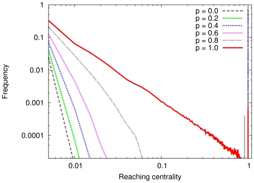
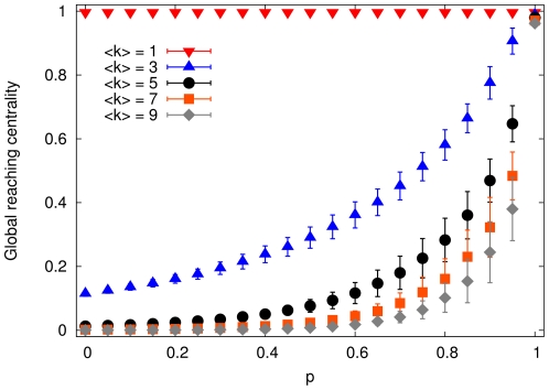
Nature, technology and society are full of complexity arising from the intricate web of the interactions among the units of the related systems (e.g., proteins, computers, people). Consequently, one of the most successful recent approaches to capturing the fundamental features of the structure and dynamics of complex systems has been the investigation of the networks associated with the above units (nodes) together with their relations (edges). Most complex systems have an inherently hierarchical organization and, correspondingly, the networks behind them also exhibit hierarchical features. Indeed, several papers have been devoted to describing this essential aspect of networks, however, without resulting in a widely accepted, converging concept concerning the quantitative characterization of the level of their hierarchy. Here we develop an approach and propose a quantity (measure) which is simple enough to be widely applicable, reveals a number of universal features of the organization of real-world networks and, as we demonstrate, is capable of capturing the essential features of the structure and the degree of hierarchy in a complex network. The measure we introduce is based on a generalization of the m-reach centrality, which we first extend to directed/partially directed graphs. Then, we define the global reaching centrality (GRC), which is the difference between the maximum and the average value of the generalized reach centralities over the network. We investigate the behavior of the GRC considering both a synthetic model with an adjustable level of hierarchy and real networks. Results for real networks show that our hierarchy measure is related to the controllability of the given system. We also propose a visualization procedure for large complex networks that can be used to obtain an overall qualitative picture about the nature of their hierarchical structure.
Overview
The claims and statistics of this paper haven’t been checked yet.
Free: it reads the open-access text and checks the first 5 claims that cite a source we can check. Create a free account to check every claim.
Integrity signals
Registry
Cites
Statistics
Figures



Verification
Claims the paper makes
The claims and statistics of this paper haven’t been checked yet.
Free: it reads the open-access text and checks the first 5 claims that cite a source we can check. Create a free account to check every claim.
Claims other papers make about this one
Each is checked against this paper’s own text: does it say what the citing paper says it does?
In the citing paper
“Awell established concept where such questions are addressed involves the use of a morphospace [32-36] namely a phenotype space where a small set of quantitative traits can be defined as the axes.”
From On the origins of hierarchy in complex networks (2013) · cites this paper as [33]
In the citing paper
“Layers can be identified through a backward or bottom up leaf removal ( LR b ) algorithm or through a forward or top down leaf removal ( LR f ) algorithm [33].”
From On the origins of hierarchy in complex networks (2013) · cites this paper as [33]
Self-check
Percentages, sums and reported differences re-computed from the paper’s own numbers.
The self-check needs the paper’s full text.
Citations
Cites
1 retracted
Retracted: Detecting Hidden Hierarchy in Terrorist Networks: Some Case Studies
Memon, N., Larsen, H. L., Hicks, D. L., & Harkiolakis, N. (2008) · Lecture notes in computer science · doi:10.1007/978-3-540-69304-8_50 · Cited by 60
Retracted(1979) · Cited by 43,841
Collective dynamics of ‘small-world’ networks
Watts, D. J., & Strogatz, S. H. (1998) · Nature · doi:10.1038/30918 · Cited by 43,060 · cited 1×
“Metabolic B is an end product of A C. elegans [48] 1173 2.442 0.048 0.052 E. coli [48] 2275 2.533 0.043 0.058 S. cerevisiae [48] 1511 2.537 0.037 0.042 Neuronal A synapse goes from A to B C. elegans [49,50] 297 7.943 0.133 0.023 Macaque brain [51] 45 10.289 0 0 Internet A communicates with B p2p-1 [52,53] 10876 3.677…”
InfluentialEmergence of Scaling in Random Networks
Barabási, A.-L., & Albert, R. (1999) · Science · doi:10.1126/science.286.5439.509 · Cited by 36,135
Statistical mechanics of complex networks
Albert, R., & Barabási, A.-L. (2002) · Reviews of Modern Physics · doi:10.1103/revmodphys.74.47 · Cited by 20,471
Community structure in social and biological networks
Girvan, M., & Newman, M. E. J. (2002) · Proceedings of the National Academy of Sciences · doi:10.1073/pnas.122653799 · Cited by 15,502
The igraph software package for complex network research
Csárdi, G., & Nepusz, T. (2006) · Medical Entomology and Zoology · Cited by 13,507
Harary, F. (1969) · Cited by 10,739
Network motifs: simple building blocks of complex networks.
Milo, R., Shen-Orr, S., Itzkovitz, S., Kashtan, N., Chklovskii, D., & Alon, U. (2002) · Science · doi:10.1126/science.298.5594.824 · Cited by 7,368
Bollobás, B. (1985) · Cited by 6,196
Research works printed but not linked: 3
- Pastor-Satorras R Vespignani A 2004 Evolution and Strcuture of the Internet Cambridge Cambridge University Press
- Healy P Nikolov NS 2004 Hierarchical drawind algorithms St Helier, NJ CRC Press
- Grinstead CM Snell JL 1997 Introduction to Probability, Second Revised Edition Washington, D.C. American Mathematical Society
Cited by
Items 101–200 of 264
Choi, I., & Kim, W. C. (2024) · International Review of Economics & Finance · doi:10.1016/j.iref.2024.103562 · Cited by 9
Nested interaction network enhances responsiveness in collective behavior
Zheng, Z., Tao, Y., Xiang, Y., Wang, T., Zhou, Y., Lei, X., Pan, G., & Peng, X. (2026) · Communications Physics · doi:10.1038/s42005-026-02510-0 · Cited by 9
Abd-Rabbo, D., & Michnick, S. W. (2017) · BMC Systems Biology · doi:10.1186/s12918-017-0418-0 · Cited by 11
Falco, D., Chowdury, A., Rosenberg, D. R., Bressler, S. L., & Diwadkar, V. A. (2020) · Brain Structure and Function · doi:10.1007/s00429-020-02061-2 · Cited by 10
Talent and experience shape competitive social hierarchies
Pósfai, M., & D’Souza, R. M. (2018) · Physical review. E · doi:10.1103/physreve.98.020302 · Cited by 10
Correction: Potential Theory for Directed Networks
Zhang, Q.-M., LinYuan, L., Wang, W., Zhu, Y.-X., & Zhou, T. (2013) · PLoS ONE · doi:10.1371/annotation/6dff4052-f7c3-4b0a-88da-85cdd5d3addd · Cited by 9
Zoo of Centralities: Encyclopedia of Node Metrics in Complex NetworksPreprint
Владимирович, Ш. С. (2025) · arXiv (Cornell University) · doi:10.48550/arxiv.2511.05122 · Cited by 11
A distributed tracing pipeline for improving locality awareness of microservices applications
Colarusso, C., De, A., Falco, I., Goglia, L., & Zimeo, E. (2024) · Software Practice and Experience · doi:10.1002/spe.3317 · Cited by 13
Complex clinical pathways of an autoimmune disease
Palla, G., Páll, N., Horváth, A., Molnár, K., Tóth, B., Kováts, T., Surján, G., Vicsek, T., & Pollner, P. (2017) · Journal of Complex Networks · doi:10.1093/comnet/cnx031 · Cited by 8
Self-citationFlorea, M., Potlog, C., Pollner, P., Abel, D., Garcia, O., Bar, S., Naqvi, S. M. A. A., & Asif, W. (2022) · River Publishers eBooks · doi:10.1201/9781003337492-9 · Cited by 8
An Improved Complexity Measure in Hierarchical Fuzzy Systems
Razak, T. R., Garibaldi, J. M., & Wagner, C. (2020) · IEEE International Conference on Fuzzy Systems (FUZZ-IEEE) · doi:10.1109/fuzz48607.2020.9177736 · Cited by 8
Modes of Interaction between Individuals Dominate the Topologies of Real World Networks
Lee, I., Kim, E., & Marcotte, E. M. (2015) · PLoS ONE · doi:10.1371/journal.pone.0121248 · Cited by 8
Existence of life in 2 + 1 dimensions
Scargill, J. H. C. (2020) · Physical Review Research · doi:10.1103/physrevresearch.2.013217 · Cited by 10
Mesoscale Modeling of Distributed Water Systems Enables Policy Search
Zhou, X., Dueñas‐Osorio, L., Doss‐Gollin, J., Liu, L., Stadler, L. B., & Li, Q. (2023) · Water Resources Research · doi:10.1029/2022wr033758 · Cited by 9
Robustness quantification of hierarchical complex networks under targeted failures
Bilal, K., Manzano, M., Erbad, A., Calle, E., & Khan, S. U. (2018) · Computers & Electrical Engineering · doi:10.1016/j.compeleceng.2018.09.008 · Cited by 10
On Using Node Indices and Their Correlations for Fake Account Detection
Asghari, S., Chehreghani, M. H., & Chehreghani, M. H. (2022) · IEEE International Conference on Big Data (BigData) · doi:10.1109/bigdata55660.2022.10020627 · Cited by 15
Social stability via management of natal males in captive rhesus macaques ( Macaca mulatta )
Pritchard, A. J., Beisner, B. A., Nathman, A. C., & McCowan, B. (2024) · Journal of Applied Animal Welfare Science · doi:10.1080/10888705.2024.2303679 · Cited by 9
End-to-End Deep Knowledge Tracing by Learning Binary Question-Embedding
Hiromi, N., Iwasawa, Y., & Matsuo, Y. (2018) · IEEE ... International Conference on Data Mining workshops · doi:10.1109/icdmw.2018.00055 · Cited by 7
Koch, F., Neutel, A., Barnes, D. K. A., Tielbörger, K., Zarfl, C., & Allhoff, K. T. (2023) · Communications Biology · doi:10.1038/s42003-023-05060-1 · Cited by 10
Revealing hidden patterns in Indian migration using network analytics
Kaur, S., Azad, S., & Gupta, A. (2024) · International Journal of Information Technology · doi:10.1007/s41870-023-01703-y · Cited by 7
Local multiresolution order in community detection
Ronhovde, P., & Nussinov, Z. (2015) · Journal of Statistical Mechanics Theory and Experiment · doi:10.1088/1742-5468/2015/01/p01001 · Cited by 7
A Measure of Structural Complexity of Hierarchical Fuzzy Systems Adapted from Software Engineering
Razak, T. R., Garibaldi, J. M., & Wagner, C. (2019) · IEEE International Conference on Fuzzy Systems (FUZZ-IEEE) · doi:10.1109/fuzz-ieee.2019.8859011 · Cited by 7
A comparative approach to quantify the heterarchical structures of complex systems
Shurety, A. L., Bodin, Ö., & Cumming, G. S. (2022) · Ecology and Society · doi:10.5751/es-13551-270338 · Cited by 7
Network analysis of the human structural connectome including the brainstem
Salhi, S., Kora, Y., Ham, G., Zadeh‐Haghighi, H., & Simon, C. (2023) · PLoS ONE · doi:10.1371/journal.pone.0272688 · Cited by 7
pyRoCS: A Python package to evaluate the resilience of complex systems
Wachtel, A., Gunda, T., Caskey, S., Cooper, R., Womack, T., Bonney, K. L., & Kliesner, K. W. (2024) · SoftwareX · doi:10.1016/j.softx.2024.101977 · Cited by 7
Vlasceanu, M., Dudík, M., & Momennejad, I. (2022) · ACM Conference on Fairness, Accountability, and Transparency (FAccT) · doi:10.1145/3531146.3533069 · Cited by 8
Germany, E., Teixeira, I., Danthine, V., Santalucia, R., Cakiroglu, I., Torres, A., Verleysen, M., Delbeke, J., Nonclercq, A., & Tahry, R. E. (2023) · Journal of Neural Engineering · doi:10.1088/1741-2552/acf1cd · Cited by 6
Hermanussen, M., Dammhahn, M., Scheffler, C., & Groth, D. (2023) · Scientific Reports · doi:10.1038/s41598-023-41225-y · Cited by 6
Higher-Order Peak Decomposition
Tan, X., Qian, J., Chen, C., Sima, Q., Wu, Y., Wang, X., & Zhang, W. (2023) · ACM International Conference on Information and Knowledge Management (CIKM) · doi:10.1145/3583780.3615209 · Cited by 6
Martino, A., Santis, E. D., Giuliani, A., & Rizzi, A. (2020) · Entropy · doi:10.3390/e22070794 · Cited by 6
Information slows down hierarchy growth
Czaplicka, A., Suchecki, K., Miñano, B., Trias, M., & Hołyst, J. A. (2014) · Physical Review E · doi:10.1103/physreve.89.062810 · Cited by 7
Comparing the Hierarchy of Keywords in On-Line News Portals
Tibély, G., Sousa-Rodrigues, D., Pollner, P., & Palla, G. (2016) · PLoS ONE · doi:10.1371/journal.pone.0165728 · Cited by 10
The Elements of Flexibility for Task-Performing Systems
Mayer, S., Sotto, L. F. D. P., & Garcke, J. (2023) · IEEE Access · doi:10.1109/access.2023.3238872 · Cited by 8
Edge Balance Ratio: Power Law From Vertices to Edges in Directed Complex Network
Wang, X., Chen, Z., Liu, P., & Gu, Y. (2013) · IEEE Journal of Selected Topics in Signal Processing · doi:10.1109/jstsp.2013.2245299 · Cited by 7
Characterization of network hierarchy reflects cell state specificity in genome organization
Wang, J., Xue, Y., He, Y., Quan, H., Zhang, J., & Gao, Y. Q. (2023) · Genome Research · doi:10.1101/gr.277206.122 · Cited by 6
Analyzing crises in global financial indices using Recurrent Neural Network based Autoencoder
Mim, M. A., Tuhin, M. K. H., & Nobi, A. (2025) · PLoS ONE · doi:10.1371/journal.pone.0326947 · Cited by 5
Exploring Influence Maximization: State-of-the-Art Methods, Taxonomies, and Trends
Meena, S. K., Singh, S. S., & Singh, K. (2025) · ACM Transactions on Knowledge Discovery from Data · doi:10.1145/3779058 · Cited by 5
Economic development and the death of the free market
Fix, B. (2021) · Evolutionary and Institutional Economics Review · doi:10.1007/s40844-021-00224-2 · Cited by 8
COVID-19 Medical Trade: Multilayer Network Analysis and Network Determinants
Peng, P., Poon, J., & Xie, X. (2023) · Networks and Spatial Economics · doi:10.1007/s11067-023-09609-9 · Cited by 5
Decision Predicate Graphs: Enhancing Interpretability in Tree Ensembles
Arrighi, L., Pennella, L., Tavares, G. M., & Barbon, S. (2024) · Communications in computer and information science · doi:10.1007/978-3-031-63797-1_16 · Cited by 13
Semantic abnormalities in schizophrenia and bipolar disorder: A natural language processing approach
Jo, Y. T., & Joo, Y. H. (2025) · Science Progress · doi:10.1177/00368504241308309 · Cited by 5
FCMiner: mining functional communities in social networks
Tennakoon, T. M. G., & Nayak, R. (2019) · Social Network Analysis and Mining · doi:10.1007/s13278-019-0565-y · Cited by 5
Biggiero, L., & Magnuszewski, R. (2021) · Advances in Complex Systems · doi:10.1142/s0219525921500120 · Cited by 5
Global excitability and network structure in the human brain
Kora, Y., Salhi, S., Davidsen, J., & Simon, C. (2023) · Physical review. E · doi:10.1103/physreve.107.054308 · Cited by 5
Social control is associated with increased reproductive skew in a wild mammal
Maldonado‐Chaparro, A. A., Philson, C. S., Zhang, X., & Blumstein, D. T. (2024) · Biology Letters · doi:10.1098/rsbl.2024.0003 · Cited by 5
Determining Team Hierarchy from Broadcast Communications
Kalia, A. K., Buchler, N., Ungvarsky, D. M., Govindan, R., & Singh, M. P. (2014) · Lecture notes in computer science · doi:10.1007/978-3-319-13734-6_35 · Cited by 5
Identifying similar networks using structural hierarchy
Saxena, R., Kaur, S., & Bhatnagar, V. (2019) · Physica A Statistical Mechanics and its Applications · doi:10.1016/j.physa.2019.04.265 · Cited by 6
An Allometric Scaling for the Number of Representative Nodes in Social Networks
Zhao, L., & Peng, T. (2020) · Springer proceedings in complexity · doi:10.1007/978-3-030-38965-9_4 · Cited by 5
Quantifying the hierarchy of public transport networks
Buijtenweg, A., Verma, T., Cats, O., Donners, B., & Wang, H. (2021) · International Conference on Models and Technologies for Intelligent Transportation Systems (MT-ITS) · doi:10.1109/mt-its49943.2021.9529271 · Cited by 5
The Ground Truth program: simulations as test beds for social science research methods
Naugle, A., Russell, A., Lakkaraju, K., Swiler, L. P., Verzi, S., & Romero, V. (2022) · Computational and Mathematical Organization Theory · doi:10.1007/s10588-021-09346-9 · Cited by 5
Khakhalin, A. S. (2019) · bioRxiv (Cold Spring Harbor Laboratory) · doi:10.1101/589887 · Cited by 5
Smith, K., Starr, J. M., Escudero, J., Ibáñez, A. M., & Parra, M. A. (2022) · Frontiers in Neuroimaging · doi:10.3389/fnimg.2022.883968 · Cited by 5
Structural complexity predicts consensus readability in online discussions
Hadfi, R., & Itō, T. (2024) · Social Network Analysis and Mining · doi:10.1007/s13278-024-01212-1 · Cited by 4
SOCIAL NETWORK ANALYSIS OF B2B NETWORKS
Mohamad, A., Wang, F., Bakar, N. A., & Jatavallabhula, P. (2017) · Universiti Utara Malaysia Institutional Repository (Universiti Utara Malaysia) · Cited by 4
The Hierarchy Structure in Directed and Undirected Signed Networks
Maktoubian, J., Noori, M., Amini, M., & Ghasempour-Mouziraji, M. (2017) · International Journal of Communications Network and System Sciences · doi:10.4236/ijcns.2017.1010012 · Cited by 6
Emergence of Leader-Follower Hierarchy Among Players in an On-Line Experiment
Toth, B. J., Palla, G., Mones, E., Havadi, G., Páll, N., Pollner, P., & Vicsek, T. (2018) · IEEE/ACM International Conference on Advances in Social Networks Analysis and Mining (ASONAM) · doi:10.1109/asonam.2018.8508278 · Cited by 7
Self-citationEvolution of hierarchy in bacterial metabolic networks
Goodman, A. J., & Feldman, M. W. (2019) · Biosystems · doi:10.1016/j.biosystems.2019.02.012 · Cited by 4
Geometric detection of hierarchical backbones in real networks
Ortiz, E., García-Pérez, G., & Serrano, M. Á. (2020) · Physical Review Research · doi:10.1103/physrevresearch.2.033519 · Cited by 5
Uncovering the geometry of protein interaction network: The case of SARS-CoV-2 protein interactome
Lecca, P. (2023) · AIP conference proceedings · doi:10.1063/5.0163052 · Cited by 4
Modeling Leadership Hierarchy in Multilevel Animal SocietiesPreprint
Ozogány, K., & Vicsek, T. (2014) · arXiv (Cornell University) · Cited by 4
Self-citationDas, D., Chaudhary, A. A., Ali, M. A. M., Alawam, A. S., Sarkar, H., & Podder, S. (2023) · FEBS Open Bio · doi:10.1002/2211-5463.13728 · Cited by 3
Hierarchy and ranking in fencing and tennis
Asztalos, B., Balázs, B., Palla, G., & Vicsek, T. (2026) · Scientific Reports · doi:10.1038/s41598-026-53459-7 · Cited by 3
Self-citationDominance, Deference, and Hierarchy Formation in Wikipedia Edit-Networks
Lerner, J., & Lomi, A. (2016) · Studies in computational intelligence · doi:10.1007/978-3-319-50901-3_8 · Cited by 3
Fitness-based growth of directed networks with hierarchy
Rodgers, N., Tiňo, P., & Johnson, S. (2024) · Journal of Physics Complexity · doi:10.1088/2632-072x/ad744e · Cited by 5
Models of random graph hierarchies
Paluch, R., Suchecki, K., & Hołyst, J. A. (2015) · The European Physical Journal B · doi:10.1140/epjb/e2015-60249-4 · Cited by 3
Measuring heterogeneity in soil networks: a network analysis and simulation-based approach
Davis, N., Polhill, G. J., & Aitkenhead, M. J. (2020) · Ecological Modelling · doi:10.1016/j.ecolmodel.2020.109308 · Cited by 3
Geometries of mixed graphs in complex vector spaces. Hierarchies and clusters in complex networks
Estrada, E. (2025) · Mathematical Modelling of Natural Phenomena · doi:10.1051/mmnp/2025009 · Cited by 3
Gene Essentiality Prediction Using Topological Features From Metabolic Networks
Nagai, J. S., Paz, H. Ê. D. S., Aono, A. H., Lorena, A. C., & Kuroshu, R. M. (2018) · Brazilian Conference on Intelligent Systems · doi:10.1109/bracis.2018.00024 · Cited by 3
Naqvi, S. M. A. A., Williams, I., Enderby, S., Pollner, P., Ábel, D., Biescas, B., García, Ó., Florea, M., & Potlog, C. (2019) · IEEE European Symposium on Security and Privacy Workshops (EuroS&PW) · doi:10.1109/eurospw.2019.00035 · Cited by 3
Exploring the gravitational model for ranking influential nodes in directed acyclic networks
Garcia‐Robledo, A., Zangiabady, M., & Sonneveld, J. (2025) · Social Network Analysis and Mining · doi:10.1007/s13278-025-01500-4 · Cited by 2
Did Shakespeare influence Seinfeld?
Date, S. (2024) · Significance · doi:10.1093/jrssig/qmae059 · Cited by 2
Topological data analysis in air traffic management: The shape of big flight data sets
Cuerno, M., Guijarro, L., Valdés, R. M. A., & Comendador, F. G. (2025) · PLoS ONE · doi:10.1371/journal.pone.0318108 · Cited by 3
Modeling rises and falls in money addicted social hierarchies
Dybiec, B., Mitarai, N., & Sneppen, K. (2014) · Physica Scripta · doi:10.1088/0031-8949/89/8/085002 · Cited by 2
Hierarchy Depth in Directed Networks
Suchecki, K., & Hołyst, J. A. (2022) · Entropy · doi:10.3390/e24020252 · Cited by 4
On the prevalence of hierarchies in social networks
Ranjbar-Sahraei, B., Ammar, H. B., Tuyls, K., & Weiß, G. (2016) · Social Network Analysis and Mining · doi:10.1007/s13278-016-0363-8 · Cited by 2
Definitions and Basic Concepts
Zafeiris, A., & Vicsek, T. (2017) · SpringerBriefs in complexity · doi:10.1007/978-3-319-70483-8_2 · Cited by 2
Self-citationA Concise Social Network Representation with Flow Hierarchy Using Frequent Interactions
Tennakoon, T. M. G., & Nayak, R. (2018) · IEEE International Conference on Tools with Artificial Intelligence (ICTAI) · doi:10.1109/ictai.2018.00101 · Cited by 2
Social Network and Organizational Leadership at the Higher Education Institution: A Case Study
Susandy, G., & Prasetyo, Y. E. (2019) · Indonesian Journal of Sustainability Accounting and Management · doi:10.28992/ijsam.v3i1.70 · Cited by 4
Cancer driver genes: a guilty by resemblance doctrine
Ramsahai, E., Tripathi, V., & John, M. (2019) · PeerJ · doi:10.7717/peerj.6979 · Cited by 2
Organisational hierarchy constructions with easy Kuramoto synchronisation
Taylor, R., Kalloniatis, A. C., & Hoek, K. (2020) · Journal of Physics A Mathematical and Theoretical · doi:10.1088/1751-8121/ab69a3 · Cited by 2
Analysis of scientific fields using journal citation networks: An empirical study
Knežević, D., & Savić, M. (2020) · International Conference on Innovations in Intelligent Systems and Applications (INISTA) · doi:10.1109/inista49547.2020.9194640 · Cited by 2
Interaction Strength Analysis to Model Retweet Cascade Graphs
Zola, P., Cola, G., Mazza, M., & Tesconi, M. (2020) · Applied Sciences · doi:10.3390/app10238394 · Cited by 14
Reyes, A. K., Salgueiro, Y., Rivera, M. E., Camargo, J. E., Hernandez, A., & Wheeler, P. W. (2021) · IEEE CHILEAN Conference on Electrical, Electronics Engineering, Information and Communication Technologies (CHILECON) · doi:10.1109/chilecon54041.2021.9703001 · Cited by 2
Recovering hierarchies in terms of content similarity
Benatti, A., & Costa, L. D. F. (2023) · Journal of Physics A Mathematical and Theoretical · doi:10.1088/1751-8121/acd3c7 · Cited by 2
Properties of Biological Networks
Dančík, V., Basu, A. B., & Clemons, P. A. (2013) · Springer eBooks · doi:10.1007/978-94-007-6803-1_5 · Cited by 4
A Hierarchy Model of Income DistributionPreprint
Fix, B. (2018) · SocArXiv (OSF Preprints) · doi:10.31235/osf.io/s3y2m · Cited by 5
Capitalist Income and Hierarchical Power: A Gradient HypothesisPreprint
Fix, B. (2018) · RePEc: Research Papers in Economics · Cited by 2
Generalised trophic levels and graph hierarchyPreprint
Moutsinas, G., Shuaib, C., Guo, W., & Jarvis, S. A. (2019) · arXiv (Cornell University) · Cited by 2
Capitalist Income and Hierarchical PowerPreprint
Fix, B. (2018) · SocArXiv (OSF Preprints) · doi:10.31235/osf.io/u8epv · Cited by 2
Network-Based Conceptualization of Observational Data
Lecca, P., Re, A., Ihekwaba, A., Mura, I., & Nguyen, T. (2016) · Elsevier eBooks · doi:10.1016/b978-0-08-100095-3.00004-4 · Cited by 1
Carbonell‐Nicolau, O. (2025) · Social Choice and Welfare · doi:10.1007/s00355-025-01582-1 · Cited by 1
Graph-Based Machine Learning Estimation Methods for Backbone Optical Network Optimization
Knapińska, A., Derda, J., Strasburger, F., Wojciechowski, S., Klikowski, J., Lechowicz, P., & Walkowiak, K. M. (2025) · IEEE Transactions on Cognitive Communications and Networking · doi:10.1109/tccn.2025.3585941 · Cited by 1
Hierarchical balance theory: Emergence of instability in follower layer below critical temperatures
Kargaran, A., Jafari, H., & Jafari, G. (2026) · Physical review. E · doi:10.1103/gdb4-5qnh · Cited by 1
Quantifying DAG-ness: A Multi-Component Framework
Csikos, E. (2026) · Northeast Journal of Complex Systems · doi:10.63562/2577-8439.1141 · Cited by 2
Romero-Naranjo, F. J. (2026) · Frontiers in Sports and Active Living · doi:10.3389/fspor.2026.1963569 · Cited by 1
Fundamental principles governing sporulation efficiency: A network theory approach
Sarkar, C., Gupta, S., Sinha, H., & Jalan, S. (2017) · Canadian Journal of Biotechnology · doi:10.24870/cjb.2017-a33 · Cited by 1
Development of a Part Criticality Index in Inventory Management
Saidy, C., Panavas, L., Harik, R., Bayoumi, A.-M., & Khoury, J. (2017) · IFIP advances in information and communication technology · doi:10.1007/978-3-319-72905-3_17 · Cited by 1
High Performance Robotic Computing as an enabler for cooperative flights
Camargo-Forero, L., Royo, P., & Prats, X. (2018) · IEEE/AIAA Digital Avionics Systems Conference (DASC) · doi:10.1109/dasc.2018.8569851 · Cited by 1
Кamola, M. (2019) · Security and Communication Networks · doi:10.1155/2019/7510809 · Cited by 1
Power in the U.S. political economy: A network analysis
Malik, N., Spencer, D., & Bui, Q. N. (2021) · Journal of the Association for Information Science and Technology · doi:10.1002/asi.24453 · Cited by 1
Metadata
- Authors
- Mones, E., Vicsek, L., & Vicsek, T.
- Affiliations
- Eötvös Loránd University (HU)
- Corvinus University of Budapest (HU)
- Corresponding author
- Vicsek, Tamás
- Venue
- PLoS ONE
- Publisher
- Public Library of Science (PLoS)
- Published
- 2012-03-28
- Volume
- 7
- Issue
- 3
- Pages
- e33799
- ISSN
- 1932-6203 (ISSN-L)
- PMC
- PMC3314676
- OpenAlex
- W2084974221
- Cited by
- 259
- References
- 69
- Citations by year
- 2026: 8 · 2025: 18 · 2024: 24 · 2023: 18 · 2022: 13 · 2021: 22 · 2020: 41 · 2019: 21 · 2018: 16 · 2017: 14 · 2016: 18 · 2015: 9 · 2014: 15 · 2013: 18 · 2012: 4
- FWCI
- 11.15
- Type
- journal article
- Language
- en
- Open access
- gold
- doi.org
- Locations
- PLoS ONE (publishedVersion, cc-by)
- PubMed Central (publishedVersion, cc-by)
- PubMed (publishedVersion)
- arXiv (Cornell University) (submittedVersion)
- RePEc: Research Papers in Economics (submittedVersion)
- DOAJ (DOAJ: Directory of Open Access Journals) (submittedVersion, cc-by-sa)
- ELTE Digital Institutional Repository (EDIT) (Eötvös Loránd University) (submittedVersion, other-oa)
- arXiv (Cornell University)
- Funders
- FP7 Ideas: European Research Council (227878)
- Topics
- Physical Sciences › Physics and Astronomy › Statistical and Nonlinear Physics › Complex Network Analysis Techniques
- Physical Sciences › Mathematics › Discrete Mathematics and Combinatorics › Graph theory and applications
- Social Sciences › Economics, Econometrics and Finance › Economics and Econometrics › Complex Systems and Time Series Analysis
- Keywords
- network hierarchy, complex networks, directed graphs, network controllability, network visualization
- MeSH terms
- Algorithms, Humans, Models, Theoretical, Neural Networks, Computer, Community Networks, Internet, Metabolic Networks and Pathways, Social Networking
About these checks
Registry, retraction, Cites and statistics results are computed, not judged, with one exception: a printed reference that no index lists is read once by a model before it counts as a citation error. Claims are extracted by a model and kept only when their quote appears verbatim in the text; each cited source is then checked, with a model’s help, for whether it says what the claim relies on. Those verdicts can be wrong — read the claim’s quote and the cited source before relying on one.
Statistics and arithmetic are recomputed, not judged.
Confidence bands are shown only for fields calibrated on our annotated test set. None is calibrated yet, so no band is shown.
What counts as a claim ›How we measure confidence ›How we check this ›
Are you an author, or do you see a problem with this page? Request a review
Data sources
Bibliographic data: Semantic Scholar, OpenAlex, Crossref.
Contains information from the Semantic Scholar Academic Graph Datasets, made available under the ODC Attribution License (ODC-BY 1.0).
Semantic Scholar’s data is described in: Kinney, R., et al. (2023). The Semantic Scholar Open Data Platform. arXiv:2301.10140.
