

The DOI matches its Crossref record; 46 of the 48 references it cites were found in a registry or an index.
Assessing robustness against potential publication bias in Activation Likelihood Estimation (ALE) meta-analyses for fMRI
Open accessAbstract
The importance of integrating research findings is incontrovertible and procedures for coordinate-based meta-analysis (CBMA) such as Activation Likelihood Estimation (ALE) have become a popular approach to combine results of fMRI studies when only peaks of activation are reported. As meta-analytical findings help building cumulative knowledge and guide future research, not only the quality of such analyses but also the way conclusions are drawn is extremely important. Like classical meta-analyses, coordinate-based meta-analyses can be subject to different forms of publication bias which may impact results and invalidate findings. The file drawer problem refers to the problem where studies fail to get published because they do not obtain anticipated results (e.g. due to lack of statistical significance). To enable assessing the stability of meta-analytical results and determine their robustness against the potential presence of the file drawer problem, we present an algorithm to determine the number of noise studies that can be added to an existing ALE fMRI meta-analysis before spatial convergence of reported activation peaks over studies in specific regions is no longer statistically significant. While methods to gain insight into the validity and limitations of results exist for other coordinate-based meta-analysis toolboxes, such as Galbraith plots for Multilevel Kernel Density Analysis (MKDA) and funnel plots and egger tests for seed-based d mapping, this procedure is the first to assess robustness against potential publication bias for the ALE algorithm. The method assists in interpreting meta-analytical results with the appropriate caution by looking how stable results remain in the presence of unreported information that may differ systematically from the information that is included. At the same time, the procedure provides further insight into the number of studies that drive the meta-analytical results. We illustrate the procedure through an example and test the effect of several parameters through extensive simulations. Code to generate noise studies is made freely available which enables users to easily use the algorithm when interpreting their results.
Overview
The claims and statistics of this paper haven’t been checked yet.
Run the check — free, no account needed. It reads the open-access text and checks the sources it cites.
Integrity signals
Registry
Cites
Statistics
Figures
Verification
Claims the paper makes
The claims and statistics of this paper haven’t been checked yet.
Run the check — free, no account needed. It reads the open-access text and checks the sources it cites.
Claims other papers make about this one
Each is checked against this paper’s own text: does it say what the citing paper says it does?
The cited source says what the claim attributes to it.
In the citing paper
“By pooling together numerous studies, ALE also allows for an increased power to detect true effects (Acar et al., 2018).”
From Bridging phenomenology and neural mechanisms of inner speech: ALE meta-analysis on egocentricity and spontaneity in a dual-mechanistic framework (2023) · cites this paper as Acar et al., 2018
Self-check
Percentages, sums and reported differences re-computed from the paper’s own numbers.
The self-check needs the paper’s full text.
Citations
Cites
Bias in meta-analysis detected by a simple, graphical test
Egger, M., Smith, G. D., Schneider, M., & Minder, C. (1997) · BMJ · doi:10.1136/bmj.315.7109.629 · Cited by 56,722 · cited 1×
“The Egger regression test estimates funnel plot asymmetry and can therefore be used as an indicator for the presence of publication bias [32].”
MethodDuval, S., & Tweedie, R. (2000) · Biometrics · doi:10.1111/j.0006-341x.2000.00455.x · Cited by 14,099 · cited 1×
“In classical meta-analysis techniques (based on summarizing effect sizes), this is for instance possible with the trim and fill method [41], that looks at the asymmetry present in a funnel plot and tries to fill the gap.”
MethodThe file drawer problem and tolerance for null results.
Rosenthal, R. (1979) · Psychological Bulletin · doi:10.1037/0033-2909.86.3.638 · Cited by 9,068 · cited 3×
“The original FSN [21] represents the required number of findings with an effect of zero to change the conclusions of the meta-analysis under the assumption that these findings are still in the “file drawer”.”
BackgroundInfluentialSterne, J. A. C., Sutton, A. J., Ioannidis, J. P. A., Terrin, N., Jones, D. R., Lau, J., Carpenter, J., Rucker, G., Harbord, R. M., Schmid, C. H., et al. (2011) · BMJ · doi:10.1136/bmj.d4002 · Cited by 7,709
Some Methods for Strengthening the Common χ 2 Tests
Cochran, W. G. (1954) · Biometrics · doi:10.2307/3001616 · Cited by 3,718
What we can do and what we cannot do with fMRI
Logothetis, N. K. (2008) · Nature · doi:10.1038/nature06976 · Cited by 3,612 · cited 1×
“Functional magnetic resonance imaging (fMRI) continues to contribute greatly to the knowledge about the location of cognitive functions in the brain [1].”
BackgroundPublication Bias in Meta‐Analysis: Prevention, Assessment and Adjustments
(2005) · doi:10.1002/0470870168 · Cited by 2,368
Eickhoff, S. B., Laird, A. R., Grefkes, C., Wang, L. E., Zilles, K., & Fox, P. T. (2009) · Human Brain Mapping · doi:10.1002/hbm.20718 · Cited by 1,924 · cited 1×
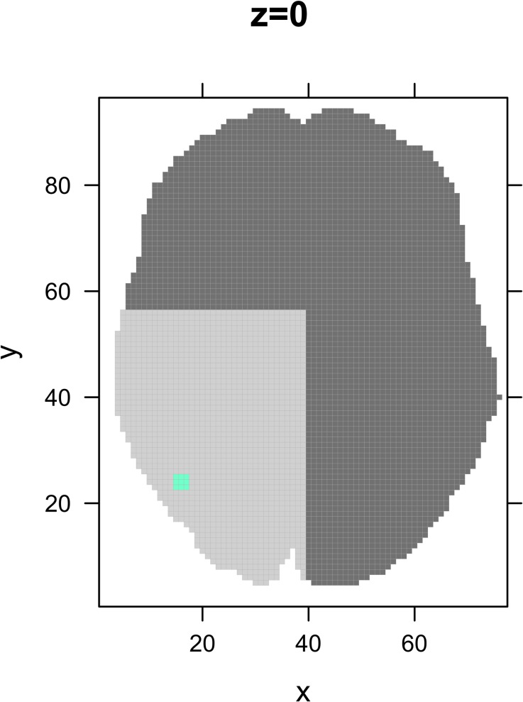
“We select a meta-analysis on finger tapping [7,38] from the BrainMap database that was used to demonstrate the working of GingerALE [15–17].”
MethodSelf-citationPublication bias in meta-analysis: Prevention, assessment and adjustments
Viechtbauer, W. (2007) · Psychometrika · doi:10.1007/s11336-006-1450-y · Cited by 1,508 · cited 3×
“We illustrate the FSN with an example from the book “Publication Bias in Meta-Analysis” [20].”
BackgroundMethodInfluentialActivation Likelihood Estimation meta-analysis revisited
Eickhoff, S., Bzdok, D., Laird, A., Kurth, F., & Fox, P. (2011) · NeuroImage · doi:10.1016/j.neuroimage.2011.09.017 · Cited by 1,448
Self-citationTurkeltaub, P., Eickhoff, S., Laird, A. R., Fox, M., Wiener, M., & Fox, P. (2011) · Human Brain Mapping · doi:10.1002/hbm.21186 · Cited by 1,114 · cited 1×
“Therefore, in this example all contrasts that stem from the same study with the same set of subjects are reported as one experiment [8].”
ResultSelf-citationVoxel-wise meta-analysis of grey matter changes in obsessive-compulsive disorder
Radua, J., & Mataix-Cols, D. (2009) · British Journal of Psychiatry · doi:10.1192/bjp.bp.108.055046 · Cited by 863 · cited 2×
“Seed-based d mapping also allows to perform sensitivity analyses using jackknife-analyses [33] or leave-one-out analyses [34] to study how replicable the original findings are.”
MethodPublication bias and clinical trials
Dickersin, K., Chan, S., Chalmersx, T. C., Sacks, H. S., & Smith, H. (1987) · Controlled Clinical Trials · doi:10.1016/0197-2456(87)90155-3 · Cited by 715 · cited 1×
“Regardless of the area of research, statistically significant findings are more likely to get published than studies with non-significant results [19] implying that the latter remain largely hidden.”
BackgroundImpact of covert duplicate publication on meta-analysis: a case study
Tramèr, M. R., Reynolds, D. J. M., Moore, R. A., & McQuay, H. J. (1997) · BMJ · doi:10.1136/bmj.315.7109.635 · Cited by 702 · cited 1×
“Using correlated data by reporting multiple experiments on the same set of subjects is problematic and induces bias [39,40].”
BackgroundEickhoff, S. B., Nichols, T. E., Laird, A. R., Hoffstaedter, F., Amunts, K., Fox, P. T., Bzdok, D., & Eickhoff, C. R. (2016) · NeuroImage · doi:10.1016/j.neuroimage.2016.04.072 · Cited by 683 · cited 10×
“The authors of the ALE algorithm advise to employ a voxel- or cluster-level family-wise error correction (FWE) [28].”
BackgroundMethodResultInfluentialSelf-citationMapping context and content: the BrainMap model
Fox, P. T., & Lancaster, J. L. (2002) · Nature reviews. Neuroscience · doi:10.1038/nrn789 · Cited by 473
The secret lives of experiments: Methods reporting in the fMRI literature
Carp, J. (2012) · NeuroImage · doi:10.1016/j.neuroimage.2012.07.004 · Cited by 463 · cited 2×
“fMRI studies exhibit great heterogeneity, stemming from the way experiments are constructed, carried out, analyzed and reported [2].”
BackgroundPublication Bias in Research Synthesis: Sensitivity Analysis Using A Priori Weight Functions.
Vevea, J. L., & Woods, C. M. (2005) · Psychological Methods · doi:10.1037/1082-989x.10.4.428 · Cited by 461 · cited 1×
“The method of Vevea and Woods [42] corrects for publication bias by adjusting weights assigned to different studies based on study characteristics that could influence likeliness of publication, such as statistical significance.”
MethodMeta-analysis of functional neuroimaging data: current and future directions
Wager, T. D., Lindquist, M., & Kaplan, L. (2007) · Social Cognitive and Affective Neuroscience · doi:10.1093/scan/nsm015 · Cited by 434 · cited 1×
“Using correlated data by reporting multiple experiments on the same set of subjects is problematic and induces bias [39,40].”
BackgroundLaird, A., Lancaster, J., & Fox, P. (2007) · Neuroinformatics · doi:10.1385/ni:3:1:065 · Cited by 379
Bradbury, K., Saboo, R., Johnson, T. L., Malof, J. M., Devarajan, A., Zhang, W.-M., Collins, L., & Newell, R. (2016) · Scientific Data · doi:10.1038/sdata.2016.106 · Cited by 370
Publication Bias (The "File-Drawer Problem") in Scientific Inference
Scargle, J. D. (1999) · arXiv · doi:10.48550/arxiv.physics/9909033 · Cited by 313
Raudenbush, S. W. (1984) · Journal of Educational Psychology · doi:10.1037/0022-0663.76.1.85 · Cited by 302 · cited 1×
“The analysis is based on a dataset from Raudenbush on teacher expectancy, a paradigm where the influence of teacher expectancy on intelligence test performance is measured [44].”
MethodExcess Significance Bias in the Literature on Brain Volume Abnormalities
Ioannidis, J. P. A. (2011) · Archives of General Psychiatry · doi:10.1001/archgenpsychiatry.2011.28 · Cited by 299 · cited 1×
“In neuroimaging literature, it has been shown that there is an excess of positive findings in literature [24, 25].”
BackgroundBrainmap taxonomy of experimental design: Description and evaluation
Fox, P. T., Laird, A. R., Fox, S. P., Fox, P. M., Uecker, A. M., Crank, M. C., Koenig, S. F., & Lancaster, J. L. (2005) · Human Brain Mapping · doi:10.1002/hbm.20141 · Cited by 297
Meta-analytic methods for neuroimaging data explained
Raduà, J., & Mataix‐Cols, D. (2012) · Biology of Mood & Anxiety Disorders · doi:10.1186/2045-5380-2-6 · Cited by 250
Evaluating the consistency and specificity of neuroimaging data using meta-analysis
Wager, T. D., Lindquist, M. A., Nichols, T. E., Kober, H., & Van Snellenberg, J. X. (2009) · NeuroImage · doi:10.1016/j.neuroimage.2008.10.061 · Cited by 242 · cited 10×
“Different algorithms have been developed to conduct a meta- PLOS ONE | https://doi.org/10.1371/journal.pone.0208177 November 30, 2018 4 / 23 analysis on peak locations and in this section, we will briefly explain the three most used, seedbased d mapping, the ALE algorithm and MKDA.”
MethodInfluentialWhite Matter Development in Adolescence: Diffusion Tensor Imaging and Meta-Analytic Results
Peters, B. D., Szeszko, P. R., Raduà, J., Ikuta, T., Gruner, P., DeRosse, P., Zhang, J., Giorgio, A., Qiu, D., Tapert, S. F., et al. (2012) · Schizophrenia Bulletin · doi:10.1093/schbul/sbs054 · Cited by 214 · cited 1×
“Seed-based d mapping also allows to perform sensitivity analyses using jackknife-analyses [33] or leave-one-out analyses [34] to study how replicable the original findings are.”
MethodMultimodal Voxel-Based Meta-Analysis of White Matter Abnormalities in Obsessive–Compulsive Disorder
Raduà, J., Grau, M., van den Heuvel, O. A., de Schotten, M. T., Stein, D. J., Canales-Rodríguez, E. J., Catani, M., & Mataix-Cols, D. (2014) · Neuropsychopharmacology · doi:10.1038/npp.2014.5 · Cited by 160
Potential Reporting Bias in Neuroimaging Studies of Sex Differences
David, S. P., Naudet, F., Laude, J. R., Raduà, J., Fusar‐Poli, P., Chu, I. M., Stefanick, M. L., & Ioannidis, J. P. A. (2018) · Scientific Reports · doi:10.1038/s41598-018-23976-1 · Cited by 140 · cited 1×
“specifically mention selective outcome and analysis reporting bias, manipulation of parameters (such as lenient thresholding) and under-reporting of null results (file drawer) [26].”
BackgroundEysenck, H., Stouffer, S., Suchman, E., DeVinney, L. C., Star, S. A., Williams, R., Lumsdaine, A. A., Lumsdaine, M. H., Smith, M. B., Janis, I., et al. (1950) · British Journal of Sociology · doi:10.2307/586897 · Cited by 133
Potential Reporting Bias in fMRI Studies of the Brain
David, S. P., Ware, J. J., Chu, I. M., Loftus, P. D., Fusar-Poli, P., Radua, J., Munafò, M. R., & Ioannidis, J. P. A. (2013) · PLoS ONE · doi:10.1371/journal.pone.0070104 · Cited by 130 · cited 1×
“In neuroimaging literature, it has been shown that there is an excess of positive findings in literature [24, 25].”
BackgroundPublication Bias in Neuroimaging Research: Implications for Meta-Analyses
Jennings, R. G., & Horn, J. D. V. (2011) · Neuroinformatics · doi:10.1007/s12021-011-9125-y · Cited by 105 · cited 2×
“While such methods could be translated to neuroimaging studies as shown in [27] for a single outcome such as brain volume or correlation between regions or to corrections at voxel-level when effect sizes are used as in seed-based d-mapping [33], extending this to settings where only peak locations instead of effect si…”
BackgroundMethodThe Usefulness of the "Fail-Safe" Statistic in Meta-Analysis
Carson, K. P., Schriesheim, C. A., & Kinicki, A. J. (1990) · Educational and Psychological Measurement · doi:10.1177/0013164490502001 · Cited by 99 · cited 2×
“The measure provides an addition to the interpretation of results because it helps in the assessment of the confidence that can be placed in them [18] by showing how stable they remain in the presence of unreported information that may differ systematically from the information that is included.”
BackgroundSharing brain mapping statistical results with the neuroimaging data model
Maumet, C., Auer, T., Bowring, A., Chen, G., Das, S., Flandin, G., Ghosh, S. S., Glatard, T., Gorgolewski, K. J., Helmer, K., et al. (2016) · Scientific Data · doi:10.1038/sdata.2016.102 · Cited by 98 · cited 1×
“000 voxels in the brain, however, the most prevailing trend to report results remains providing only the coordinates of statistically significant local maxima (called peaks or foci) [6].”
BackgroundKiciński, M. (2014) · BMJ Open · doi:10.1136/bmjopen-2014-004831 · Cited by 72
Meta Analysis of Functional Neuroimaging Data via Bayesian Spatial Point Processes
Kang, J., Johnson, T., Nichols, T. E., & Wager, T. (2011) · Journal of the American Statistical Association · doi:10.1198/jasa.2011.ap09735 · Cited by 68
Modeling motor connectivity using TMS/PET and structural equation modeling
Laird, A., Robbins, J. M., Li, K., Price, L. R., Cykowski, M., Narayana, S., Laird, R. W., Franklin, C., & Fox, P. (2008) · NeuroImage · doi:10.1016/j.neuroimage.2008.01.065 · Cited by 55 · cited 1×
“We select a meta-analysis on finger tapping [7,38] from the BrainMap database that was used to demonstrate the working of GingerALE [15–17].”
MethodPost-hoc power estimation for topological inference in fMRI
Durnez, J., Moerkerke, B., & Nichols, T. E. (2014) · NeuroImage · doi:10.1016/j.neuroimage.2013.07.072 · Cited by 36 · cited 1×
“Furthermore, fMRI studies are relatively expensive which often limits the size of studies [2] leading to low statistical power to detect true activation [3].”
BackgroundSelf-citationMeta-analysis of functional neuroimaging data using Bayesian nonparametric binary regression
Yue, Y., Lindquist, M., & Loh, J. (2012) · The Annals of Applied Statistics · doi:10.1214/11-aoas523 · Cited by 34
A BAYESIAN HIERARCHICAL SPATIAL POINT PROCESS MODEL FOR MULTI-TYPE NEUROIMAGING META-ANALYSIS
Kang, J., Nichols, T. E., Wager, T., & Johnson, T. (2014) · Annals of Applied Statistics · doi:10.1214/14-aoas757 · Cited by 33
Fail-Safe Ns for One- Versus Two-Tailed Tests Lead to Different Conclusions About Publication Bias
Hsu, L. (2002) · Understanding Statistics · doi:10.1207/s15328031us0102_02 · Cited by 24 · cited 1×
“This was later adapted by Hsu [23] to the maximum number of studies with nonsignificant findings that can be added to a meta-analysis before the conclusions no longer hold.”
BackgroundRowe, F. J., Barton, P. G., Bedson, E., Breen, R., Conroy, E., Cwiklinski, E., Dodridge, C., Drummond, A., García-Fiñana, M., Howard, C., et al. (2014) · BMJ Open · doi:10.1136/bmjopen-2014-005885 · Cited by 21
A Generalized Publication Bias ModelPreprint
Schönemann, P. H., & Scargle, J. D. (2008) · arXiv (Cornell University) · doi:10.6129/cjp.2008.5001.02 · Cited by 16
Estimating the prevalence of missing experiments in a neuroimaging meta-analysisPreprint
Samartsidis, P., Montagna, S., Laird, A. R., Fox, P. T., Johnson, T. D., & Nichols, T. E. (2017) · bioRxiv (Cold Spring Harbor Laboratory) · doi:10.1101/225425 · Cited by 9 · cited 4×
“A recent paper estimates the number of studies or experiments with no foci that remain unnoticed in fMRI meta-analyses [37].”
BackgroundMethodResultInfluentialTime-warped growth processes, with applications to the modeling of boom-bust cycles in house prices
Peng, J., Paul, D., & Müller, H.-G. (2014) · doi:10.1214/14-aoas740 · Cited by 8
Research works printed but not linked: 3
- J Radua, 2012, Meta-analytic methods for neuroimaging data explained, Biology of Mood & Anxiety Disorders, 2, 1
- SG Costafreda, 2012, Parametric coordinate-based meta-analysis: Valid effect size meta-analysis of studies with differing statistical thresholds, Journal of Neuroscience Methods, 210, 291, 10.1016/j.jneumeth.2012.07.016 · DOI
- A Laird, 2008, Brainmap: The social evolution of a functional neuroimaging database, Neuroinformatics, 65
Cited by
Sorted by citations
Gray, J. P., Müller, V. I., Eickhoff, S. B., & Fox, P. T. (2020) · American Journal of Psychiatry · doi:10.1176/appi.ajp.2019.19050560 · Cited by 449
“(15) to estimate the robustness of identified results against unpublished neuroimaging findings.”
BackgroundMethodSelf-citationPando‐Naude, V., Toxto, S., Fernandez‐Lozano, S., Parsons, C. E., Alcauter, S., & Garza‐Villarreal, E. A. (2021) · Translational Psychiatry · doi:10.1038/s41398-020-01128-2 · Cited by 195
Current Challenges in Translational and Clinical fMRI and Future Directions
Specht, K. (2020) · Frontiers in Psychiatry · doi:10.3389/fpsyt.2019.00924 · Cited by 130
The Neural Correlates of Time: A Meta-analysis of Neuroimaging Studies
Nani, A., Manuello, J., Liloia, D., Duca, S., Costa, T., & Cauda, F. (2019) · Journal of Cognitive Neuroscience · doi:10.1162/jocn_a_01459 · Cited by 109
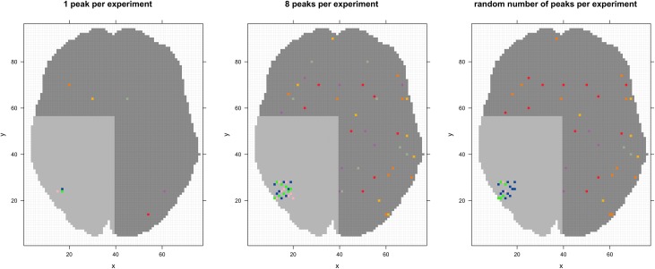
“Noise experiments are then created randomly by combining values of sample size and amount of reported foci per experiment taken from the respective real distributions (Acar et al., 2018).”
BackgroundMethodInfluentialAntoniou, G., Lambourg, E. J., Steele, J. D., & Colvin, L. (2023) · British Journal of Anaesthesia · doi:10.1016/j.bja.2023.03.008 · Cited by 133
“Thus, traditional measures of heterogeneity are not applicable.(141,143,144) Second, the limited number of neuro-”
Background
Metadata
- Authors
- Acar, F., Seurinck, R., Eickhoff, S. B., & Moerkerke, B.
- Affiliations
- Ghent University (BE)
- Forschungszentrum Jülich (DE)
- Corresponding author
- Acar, Freya
- Venue
- PLOS ONE
- Publisher
- Public Library of Science (PLoS)
- Published
- 2018-11-30
- Volume
- 13
- Issue
- 11
- Pages
- e0208177
- ISSN
- 1932-6203 (ISSN-L)
- PMC
- PMC6267999
- OpenAlex
- W2902120147
- Cited by
- 154
- References
- 48
- Citations by year
- 2026: 22 · 2025: 19 · 2024: 18 · 2023: 28 · 2022: 27 · 2021: 19 · 2020: 13 · 2019: 7
- FWCI
- 7.44
- Type
- journal article
- Language
- en
- Open access
- gold
- doi.org
- Licence
- Locations
- PLoS ONE (publishedVersion, cc-by)
- Europe PMC (PubMed Central) (publishedVersion, cc-by)
- PubMed Central (publishedVersion, cc-by)
- PubMed (publishedVersion)
- Ghent University Academic Bibliography (Ghent University) (submittedVersion, other-oa)
- RePEc: Research Papers in Economics (submittedVersion)
- DOAJ (DOAJ: Directory of Open Access Journals) (submittedVersion, cc-by-sa)
- JuSER (Forschungszentrum Jülich) (submittedVersion, other-oa)
- Funders
- Fonds Wetenschappelijk Onderzoek (G.0149.14)
- National Institute of Mental Health (R01-MH074457)
- Horizon 2020 (7202070 (HBP SGA1))
- Topics
- Social Sciences › Decision Sciences › Statistics, Probability and Uncertainty › Meta-analysis and systematic reviews
- Life Sciences › Neuroscience › Cognitive Neuroscience › Functional Brain Connectivity Studies
- Social Sciences › Psychology › Experimental and Cognitive Psychology › Psychology Research and Bibliometrics
- Keywords
- publication bias, file drawer problem, activation likelihood estimation, coordinate-based meta-analysis, noise study, robustness analysis, spatial convergence
- MeSH terms
- Algorithms, Brain, Brain Mapping, Humans, Magnetic Resonance Imaging, Meta-Analysis as Topic, Likelihood Functions, Publication Bias
About these checks
Registry, retraction, Cites and statistics results are computed, not judged, with one exception: a printed reference that no index lists is read once by a model before it counts as a citation error. Claims are extracted by a model and kept only when their quote appears verbatim in the text; each cited source is then checked, with a model’s help, for whether it says what the claim relies on. Those verdicts can be wrong — read the claim’s quote and the cited source before relying on one.
Statistics and arithmetic are recomputed, not judged.
Confidence bands are shown only for fields calibrated on our annotated test set. None is calibrated yet, so no band is shown.
What counts as a claim ›How we measure confidence ›How we check this ›
Are you an author, or do you see a problem with this page? Request a review
