

The DOI matches its Crossref record; 44 of the 44 references it cites were found in a registry or an index.
Attention Modulates the Responses of Simple Cells in Monkey Primary Visual Cortex
Open accessAbstract
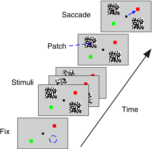
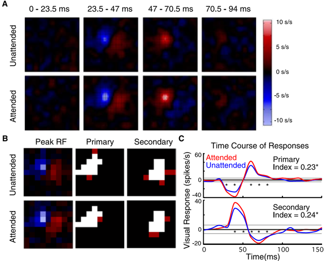
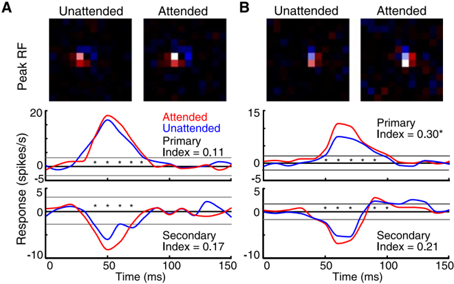
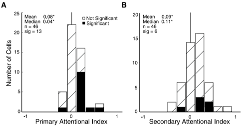
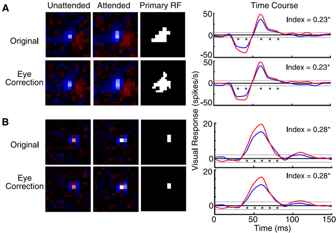
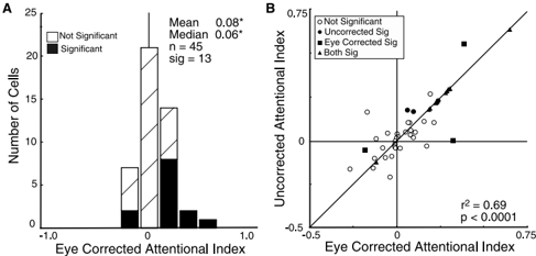
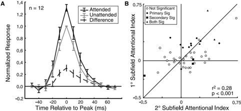
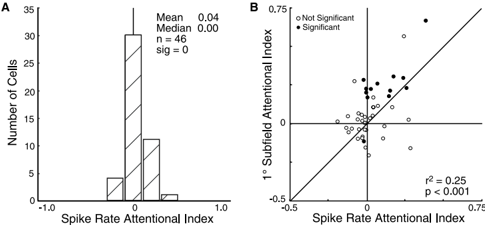
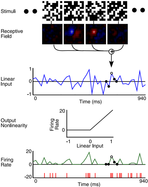
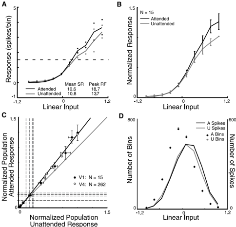
Spatial attention has long been postulated to act as a spotlight that increases the salience of visual stimuli at the attended location. We examined the effects of attention on the receptive fields of simple cells in primary visual cortex (V1) by training macaque monkeys to perform a task with two modes. In the attended mode, the stimuli relevant to the animal's task overlay the receptive field of the neuron being recorded. In the unattended mode, the animal was cued to attend to stimuli outside the receptive field of that neuron. The relevant stimulus, a colored pixel, was briefly presented within a white-noise stimulus, a flickering grid of black and white pixels. The receptive fields of the neurons were mapped by correlating spikes with the white-noise stimulus in both attended and unattended modes. We found that attention could cause significant modulation of the visually evoked response despite an absence of significant effects on the overall firing rates. On further examination of the relationship between the strength of the visual stimulation and the firing rate, we found that attention appears to cause multiplicative scaling of the visually evoked responses of simple cells, demonstrating that attention reaches back to the initial stages of visual cortical processing.
Overview
The claims and statistics of this paper haven’t been checked yet.
Run the check — free, no account needed. It reads the open-access text and checks the sources it cites.
Integrity signals
Registry
Cites
Statistics
Figures
Verification
Claims the paper makes
The claims and statistics of this paper haven’t been checked yet.
Run the check — free, no account needed. It reads the open-access text and checks the sources it cites.
Claims other papers make about this one
Each is checked against this paper’s own text: does it say what the citing paper says it does?
In the citing paper
“Attentional modulation of neural gain has been particularly well studied in the non-human primate visual system1,42,43, in which visual spatial attention within the receptive field of a recorded neuron enhances both contrast gain (that is, scaling of that neuron’s stimulus-response relationship along the contrast axis)43 and response gain (that is, multiplicative transformation of responses to all”
From Mechanisms underlying gain modulation in the cortex (2020) · cites this paper as [42]
Self-check
Percentages, sums and reported differences re-computed from the paper’s own numbers.
The self-check needs the paper’s full text.
Citations
Cites
Receptive fields, binocular interaction and functional architecture in the cat’s visual cortex
Hubel, D. H., & Wiesel, T. N. (1962) · The Journal of Physiology · doi:10.1113/jphysiol.1962.sp006837 · Cited by 13,680
Receptive fields and functional architecture of monkey striate cortex
Hubel, D. H., & Wiesel, T. N. (1968) · The Journal of Physiology · doi:10.1113/jphysiol.1968.sp008455 · Cited by 6,685
Attention and the detection of signals.
Posner, M. I., Snyder, C. R., & Davidson, B. J. (1980) · Journal of Experimental Psychology: General · doi:10.1037/0096-3445.109.2.160 · Cited by 3,778
Gorillas in our midst: sustained inattentional blindness for dynamic events
Simons, D. J., & Chabris, C. F. (1999) · Perception · doi:10.1068/p281059 · Cited by 3,181
Selective Attention Gates Visual Processing in the Extrastriate Cortex
Moran, J., & Desimone, R. (1985) · Science · doi:10.1126/science.4023713 · Cited by 2,433
Selective Attention Gates Visual Processing in the Extrastriate Cortex
Moran, J., & Desimone, R. (2003) · The MIT Press eBooks · doi:10.7551/mitpress/2834.003.0024 · Cited by 2,164
Neural mechanisms of spatial selective attention in areas V1, V2, and V4 of macaque visual cortex
Luck, S. J., Chelazzi, L., Hillyard, S. A., & Desimone, R. (1997) · Journal of Neurophysiology · doi:10.1152/jn.1997.77.1.24 · Cited by 1,615
Feature-based attention influences motion processing gain in macaque visual cortex
Treue, S., & Trujillo, J. C. M. (1999) · Nature · doi:10.1038/21176 · Cited by 1,465
Effects of Attention on Orientation-Tuning Functions of Single Neurons in Macaque Cortical Area V4
McAdams, C. J., & Maunsell, J. H. R. (1999) · Journal of Neuroscience · doi:10.1523/jneurosci.19-01-00431.1999 · Cited by 1,218
Self-citationMotter, B. C. (1993) · Journal of Neurophysiology · doi:10.1152/jn.1993.70.3.909 · Cited by 1,055
Research works printed but not linked: 1
- 1981, Exp Brain Res, 44, 213
Cited by
Sorted by citations
Items 101–200 of 203
Dynamic communication of attention signals between the LGN and V1
Mock, V. L., Luke, K. L., Hembrook‐Short, J. R., & Briggs, F. (2018) · Journal of Neurophysiology · doi:10.1152/jn.00224.2018 · Cited by 18
Adamian, N., & Andersen, . K. (2023) · Journal of Cognitive Neuroscience · doi:10.1162/jocn_a_02070 · Cited by 17
Hamilton, R. H., Stark, M., & Coslett, H. B. (2009) · Cortex · doi:10.1016/j.cortex.2009.02.005 · Cited by 17
The effect of aging on the spatial frequency selectivity of the human visual system
Govenlock, S. W., Taylor, C. P., Sekuler, A. B., & Bennett, P. (2010) · Vision Research · doi:10.1016/j.visres.2010.05.025 · Cited by 17
A two-stage neural spiking model of visual contrast detection in perimetry
Gardiner, S. K., Swanson, W. H., Demirel, S., McKendrick, A. M., Turpin, A. H., & Johnson, C. A. (2008) · Vision Research · doi:10.1016/j.visres.2008.06.006 · Cited by 17
Mohr, K. S., Carr, N., Georgel, R., & Kelly, S. P. (2020) · Cerebral Cortex Communications · doi:10.1093/texcom/tgaa045 · Cited by 16
An Attempt at a Unified Theory of the Neocortical Microcircuit in Sensory Cortex
Bennett, M. S. (2020) · Frontiers in Neural Circuits · doi:10.3389/fncir.2020.00040 · Cited by 16
Fagioli, S., & Macaluso, E. (2008) · Journal of Cognitive Neuroscience · doi:10.1162/jocn.2009.21116 · Cited by 15
Neural Mechanisms of Attention
Cohen, R. A. (2013) · Springer eBooks · doi:10.1007/978-0-387-72639-7_10 · Cited by 15
Fu, S., Fedota, J. R., Greenwood, P. M., & Parasuraman, R. (2012) · Biological Psychology · doi:10.1016/j.biopsycho.2012.03.012 · Cited by 14
Curtis, M. T., Ren, X., Coffman, B. A., & Salisbury, D. F. (2022) · Human Brain Mapping · doi:10.1002/hbm.26067 · Cited by 12
Stable bottom‐up processing during dynamic top‐down modulations in monkey auditory cortex
Massoudi, R., van Wanrooij, M. M., Wetter, S. M. C. I. V., Versnel, H., & Opstal, A. J. V. (2013) · European Journal of Neuroscience · doi:10.1111/ejn.12180 · Cited by 13
Modulation of neuronal responses in macaque primary visual cortex in a memory task
Vidyasagar, T. R., & Pigarev, I. N. (2007) · European Journal of Neuroscience · doi:10.1111/j.1460-9568.2007.05483.x · Cited by 13
Neural mechanisms of resource allocation in working memory
Li, H.-H., Sprague, T. C., Yoo, A. H., Ma, W. J., & Curtis, C. E. (2025) · Science Advances · doi:10.1126/sciadv.adr8015 · Cited by 12
Barbot, A., Landy, M. S., & Carrasco, M. (2012) · Journal of Vision · doi:10.1167/12.8.6 · Cited by 12
The role of the thalamic reticular nucleus in visual processing
Sillito, A. M., & Jones, H. E. (2007) · Thalamus & Related Systems · doi:10.1017/s1472928807000295 · Cited by 12
Exploring Thalamocortical Interactions
Sherman, S. M., & Usrey, W. M. (2021) · Oxford University Press eBooks · doi:10.1093/med/9780197503874.001.0001 · Cited by 14
Griffeth, V. E. M., Simon, A. B., & Buxton, R. B. (2014) · NeuroImage · doi:10.1016/j.neuroimage.2014.10.003 · Cited by 11
Information persistence evaluated with low-density dot patterns
Greene, E. G. (2016) · Acta Psychologica · doi:10.1016/j.actpsy.2016.08.005 · Cited by 10
Neural Mechanisms of Saliency, Attention, and Orienting
White, B. J., & Munoz, D. P. (2016) · Cognitive science and technology · doi:10.1007/978-981-10-0213-7_1 · Cited by 10
Relation Between Event-Related Potential Latency and Saccade Latency in Overt Shifts of Attention
Kulke, L., Atkinson, J., & Braddick, O. (2020) · Perception · doi:10.1177/0301006620911869 · Cited by 10
Clark, K., Noudoost, B., & Moore, T. (2014) · Journal of Cognitive Neuroscience · doi:10.1162/jocn_a_00599 · Cited by 8
Spatial attention in area V4 is mediated by circuits in primary visual cortex
Tiesinga, P. H. E., & Buia, C. (2009) · Neural Networks · doi:10.1016/j.neunet.2009.07.010 · Cited by 10
Information processing bottlenecks in macaque posterior parietal cortex: an attentional blink?
Maloney, R. T., Jayakumar, J., Levichkina, E. V., Pigarev, I. N., & Vidyasagar, T. R. (2013) · Experimental Brain Research · doi:10.1007/s00221-013-3569-2 · Cited by 9
Delayed effects of attention in visual cortex as measured with fMRI
Bouvier, S. E., & Engel, S. A. (2011) · NeuroImage · doi:10.1016/j.neuroimage.2011.04.012 · Cited by 9
Spatial attention modulates earliest visual processing: An electrical neuroimaging study
Zani, A., & Proverbio, A. M. (2020) · Heliyon · doi:10.1016/j.heliyon.2020.e05570 · Cited by 9
Pan, W., Zhao, Y., Luo, Z., Chen, Y., & Cai, Y. (2023) · Psychophysiology · doi:10.1111/psyp.14507 · Cited by 8
Shah, S., Mancarella, M., Hembrook‐Short, J. R., Mock, V. L., & Briggs, F. (2021) · The Journal of Comparative Neurology · doi:10.1002/cne.25168 · Cited by 8
Physically activated modes of attentional control
Giesbrecht, B., Bullock, T., & Garrett, J. (2024) · Trends in Cognitive Sciences · doi:10.1016/j.tics.2024.11.006 · Cited by 9
Mechanisms for shaping receptive field in monkey area TE
Obara, K., O’Hashi, K., & Tanifuji, M. (2017) · Journal of Neurophysiology · doi:10.1152/jn.00348.2017 · Cited by 7
Attentional modulation of unconscious inhibitory visuomotor processes: An EEG study
Wang, Y., Di, M., Zhao, J., Hu, S., Yao, Z., & Wang, Y. (2020) · Psychophysiology · doi:10.1111/psyp.13561 · Cited by 7
Gabor feature processing in spiking neural networks from retina-inspired data
Tsitiridis, A., Conde, C., de Diego, I. M., Sáez, J. S. D. R., Gomez, J. R., & Cabello, E. (2015) · International Joint Conference on Neural Networks (IJCNN) · doi:10.1109/ijcnn.2015.7280352 · Cited by 7
Levichkina, E. V., Saalmann, Y. B., & Vidyasagar, T. R. (2017) · Physiological Reports · doi:10.14814/phy2.13136 · Cited by 8
Behavioral modulations can alter the visual tuning of neurons in the mouse thalamocortical pathway
Socha, K. Z., Couto, J., Whiteway, M. R., Hosseinjany, S., Butts, D. A., & Bonin, V. (2024) · Cell Reports · doi:10.1016/j.celrep.2024.114947 · Cited by 6
Wei, H., Ren, Y., & Wang, Z. Y. (2012) · Cognitive Neurodynamics · doi:10.1007/s11571-012-9235-8 · Cited by 6
Adaptive Gain Modulation in V1 Explains Contextual Modifications during Bisection Learning
Schäfer, R., Vasilaki, E., & Senn, W. (2009) · PLoS Computational Biology · doi:10.1371/journal.pcbi.1000617 · Cited by 6
Bio-Inspired Presentation Attack Detection for Face Biometrics
Tsitiridis, A., Conde, C., Gómez-Ayllón, B., & Cabello, E. (2019) · Frontiers in Computational Neuroscience · doi:10.3389/fncom.2019.00034 · Cited by 5
Attention: Control in the Visual Cortex
Mangun, G. R., & Fannon, S. P. (2007) · Current Biology · doi:10.1016/j.cub.2006.12.028 · Cited by 5
Networks for Attentional Control and Selection in Spatial Vision
Mangun, G. R., & Fannon, S. P. (2007) · Springer eBooks · doi:10.1007/978-0-387-71978-8_21 · Cited by 5
Feature interference as a neuronal basis for the behavioural cost of task uncertaintyPreprint
Xue, C., Markman, S. K., Chen, R., Kramer, L. E., & Cohen, M. R. (2024) · bioRxiv (Cold Spring Harbor Laboratory) · doi:10.1101/2024.03.04.583375 · Cited by 5
The Nature of Attentional Modulation in V1
Slotnick, S. D. (2013) · doi:10.1007/978-1-137-27236-2_3 · Cited by 4
Sharafeldin, A., Mock, V. L., Meisenhelter, S., Hembrook‐Short, J. R., & Briggs, F. (2020) · Cerebral Cortex Communications · doi:10.1093/texcom/tgaa014 · Cited by 3
Modeling the top-down influences on the lateral interactions in the visual cortex
Šetić, M., & Domijan, D. (2008) · Brain Research · doi:10.1016/j.brainres.2008.05.076 · Cited by 3
Tiesinga, P. H. E., & Buia, C. (2006) · arXiv (Cornell University) · doi:10.48550/arxiv.q-bio/0611030 · Cited by 3
Behavioral response to visual motion impacts population coding in the mouse visual thalamusPreprint
Socha, K. Z., Whiteway, M. R., Butts, D. A., & Bonin, V. (2018) · bioRxiv (Cold Spring Harbor Laboratory) · doi:10.1101/382671 · Cited by 3
Distributed context-dependent choice information in mouse dorsal-parietal cortexPreprint
Orlandi, J. G., Abdolrahmani, M., Aoki, R., Lyamzin, D. R., & Benucci, A. (2021) · bioRxiv (Cold Spring Harbor Laboratory) · doi:10.1101/2021.03.02.433657 · Cited by 3
Spike Timing and Thalamocortical Interactions
Usrey, W. M., & Sherman, S. M. (2021) · Oxford University Press eBooks · doi:10.1093/med/9780197503874.003.0010 · Cited by 2
What the Neuroscience and Psychology of Magic Reveal about Misinformation
Alexander, R. G., Macknik, S. L., & Martínez‐Conde, S. (2022) · Publications · doi:10.3390/publications10040033 · Cited by 4
Hierarchical organization of the forebrain cholinergic system in rats
Varsanyi, P., Alloway, K. D., Chavez, C. M., Gielow, M. R., Gombkötő, P., Kondo, H., Nádasdy, Z., & Záborszky, L. (2025) · iScience · doi:10.1016/j.isci.2025.112001 · Cited by 3
Modulation of Synchrony by Interneurons
Tiesinga, P. H. E., & Buia, C. (2008) · Elsevier eBooks · doi:10.1016/b978-012373649-9.50024-7 · Cited by 2
Neuroimaging Approaches to the Study of Visual Attention
Mangun, G. R., Liu, Y., Bengson, J. J., Fannon, S. P., DiQuattro, N. E., & Geng, J. J. (2016) · Neuromethods · doi:10.1007/978-1-4939-5611-1_13 · Cited by 2
Correction: Divisive Gain Modulation with Dynamic Stimuli in Integrate-and-Fire Neurons
Ly, C., & Doiron, B. (2009) · PLoS Computational Biology · doi:10.1371/annotation/9c4474f6-e58e-41ea-af4b-090bbb86f474 · Cited by 2
Visuelle Aufmerksamkeit: Von Orten, Eigenschaften und Kontrasten
Treue, S., Womelsdorf, T., & Martínez-Trujillo, J. (2007) · e-Neuroforum · doi:10.1515/nf-2007-0204 · Cited by 2
Attentional Modulation of Macaque Visual Processing AreasPreprint
Patel, G. H., Snyder, L. H., & Corbetta, M. (2018) · bioRxiv (Cold Spring Harbor Laboratory) · doi:10.1101/345439 · Cited by 2
Wyrick, D. G., Cain, N., Larsen, R. S., Lecoq, J. A., Valley, M. T., Ahmed, R., Bowlus, J., Boyer, G., Caldejon, S., Casal, L., et al. (2023) · bioRxiv (Cold Spring Harbor Laboratory) · doi:10.1101/2023.06.02.543483 · Cited by 2
Spatial Attention Weakly Modulates Visual Responses in the Lateral Geniculate Nucleus
Alitto, H. J., Johnson, J. S., & Usrey, W. M. (2025) · eNeuro · doi:10.1523/eneuro.0153-25.2025 · Cited by 1
Computing the effects of excitatory-inhibitory balance on neuronal input-output properties
Reyes, A. D. (2026) · PLoS Computational Biology · doi:10.1371/journal.pcbi.1013958 · Cited by 2
First and Higher Order Thalamic Relays
Usrey, W. M., & Sherman, S. M. (2021) · Oxford University Press eBooks · doi:10.1093/med/9780197503874.003.0006 · Cited by 1
Glutamatergic Drivers and Modulators
Usrey, W. M., & Sherman, S. M. (2021) · Oxford University Press eBooks · doi:10.1093/med/9780197503874.003.0005 · Cited by 1
A proposed attention-based model for spatial memory formation and retrieval
Soyer, Ç. (2022) · Cognitive Processing · doi:10.1007/s10339-022-01121-1 · Cited by 1
Yu, H., Chen, S., Ye, Z., Zhang, Q., Tu, Y., & Hua, T. (2023) · Cerebral Cortex · doi:10.1093/cercor/bhad344 · Cited by 1
Neuroimaging Approaches to the Study of Visual Attention
Mangun, G. R., Liu, Y., Bengson, J. J., Fannon, S. P., DiQuattro, N. E., Geng, J. J., Mistri, D., Tedone, N., Rocca, M. A., & Filippi, M. (2025) · Neuromethods · doi:10.1007/978-1-0716-4438-6_14 · Cited by 1
Cell Types in the Thalamus and Cortex
Usrey, W. M., & Sherman, S. M. (2021) · Oxford University Press eBooks · doi:10.1093/med/9780197503874.003.0002 · Cited by 1
Imaging Brain Attention Systems: Control and Selection in Vision
Mangun, G. R., Fannon, S. P., Geng, J. J., & Saron, C. D. (2009) · Neuromethods · doi:10.1007/978-1-60327-919-2_12 · Cited by 1
The Relationship between Attention and Rapport in Conversation with AAC Users
Nguyen, D. M. (2016) · Cited by 1
Top-Down Feedback Controls Spatial Summation and Response Gain in Primate Visual CortexPreprint
Nurminen, L., Merlin, S., Bijanzadeh, M., Federer, F., & Angelucci, A. (2016) · bioRxiv (Cold Spring Harbor Laboratory) · doi:10.1101/094680 · Cited by 1
Functional architecture of the forebrain cholinergic system in rodentsPreprint
Záborszky, L., Varsanyi, P., Alloway, K. D., Chavez, C. M., Gielow, M. R., Gombkötő, P., Kondo, H., & Nádasdy, Z. (2024) · Research Square · doi:10.21203/rs.3.rs-4504727/v1 · Cited by 1
Effects of Selective Attention on Sensory Processing of Visual Motion
Busse, L. (2006) · eDiss (Georg-August-Universität Göttingen) · doi:10.53846/goediss-180
Villalobos, C. A. (2010) · Human Biology
Banerjee, S. (2014) · CUNY Academic Works (City University of New York)
Modulation of orientation-selective neurons by motion: when additive, when multiplicative?
dge, T. L. ⁄., Urbanczik, R., & Senn, W. (2014) · Frontiers in Computational Neuroscience · doi:10.3389/fncom.2014.00067
Competition between visual stimuli in the monkey parietal cortex
Falkner, A. L. (2012) · doi:10.7916/d8794bpx
Adaptation and attention in higher visual perception
Kaping, D. (2009)
Neural and Psychological Mechanisms of Interference Control.
Nee, D. E. (2008)
Transformation of population code from dLGN to V1 facilitates linear decodingPreprint
Cayco-Gajic, N. A., Durand, S., Buice, M. A., Iyer, R., Reid, C., Zylberberg, J., & Shea‐Brown, E. (2019) · bioRxiv (Cold Spring Harbor Laboratory) · doi:10.1101/826750
Advances in the physiology of primary visual cortex in primates
Hawken, M. J. (2020) · Current Opinion in Physiology · doi:10.1016/j.cophys.2020.07.005
花沢, 明. (2006) · JOURNAL OF THE ILLUMINATING ENGINEERING INSTITUTE OF JAPAN · doi:10.2150/jieij.90.581_2
Corticothalamic Circuits Linking Sensation and Action
Usrey, W. M., & Sherman, S. M. (2021) · Oxford University Press eBooks · doi:10.1093/med/9780197503874.003.0013
Usrey, W. M., & Sherman, S. M. (2021) · Oxford University Press eBooks · doi:10.1093/med/9780197503874.003.0007
Classification of Thalamocortical and Corticothalamic Motifs
Usrey, W. M., & Sherman, S. M. (2021) · Oxford University Press eBooks · doi:10.1093/med/9780197503874.003.0009
Usrey, W. M., & Sherman, S. M. (2021) · Oxford University Press eBooks · doi:10.1093/med/9780197503874.003.0003
Brief Overview of Cortical Organization
Usrey, W. M., & Sherman, S. M. (2021) · Oxford University Press eBooks · doi:10.1093/med/9780197503874.003.0008
Parallel Processing of Sensory Signals to Cortex
Usrey, W. M., & Sherman, S. M. (2021) · Oxford University Press eBooks · doi:10.1093/med/9780197503874.003.0011
Thalamocortical Substrates of Attention
Usrey, W. M., & Sherman, S. M. (2021) · Oxford University Press eBooks · doi:10.1093/med/9780197503874.003.0012
Usrey, W. M., & Sherman, S. M. (2021) · Oxford University Press eBooks · doi:10.1093/med/9780197503874.003.0004
Usrey, W. M., & Sherman, S. M. (2021) · Oxford University Press eBooks · doi:10.1093/med/9780197503874.003.0001
Usrey, W. M., & Sherman, S. M. (2021) · Oxford University Press eBooks · doi:10.1093/med/9780197503874.003.0014
Resolution of Attention Matches the Sensory Resolution of Visual CortexPreprint
Ghose, G. M., Warren, S. G., & Kiani, A. (2022) · SSRN Electronic Journal · doi:10.2139/ssrn.4121842
Resolution of Attention Matches the Sensory Resolution of Visual CortexPreprint
Warren, S. G., Kiani, A., & Ghose, G. M. (2022) · SSRN Electronic Journal · doi:10.2139/ssrn.4121837
Usrey, W. M., & Sherman, S. M. (2021) · Oxford University Press eBooks · doi:10.1093/med/9780197503874.002.0004
Usrey, W. M., & Sherman, S. M. (2021) · Oxford University Press eBooks · doi:10.1093/med/9780197503874.002.0006
Usrey, W. M., & Sherman, S. M. (2021) · Oxford University Press eBooks · doi:10.1093/med/9780197503874.002.0003
Shafiei, M., Reik, M., Görner, M., Taubert, N., Giese, M. A., & Thier, P. (2025) · bioRxiv (Cold Spring Harbor Laboratory) · doi:10.1101/2025.07.07.663380
Silva, T. O. (2013) · LA Referencia (Red Federada de Repositorios Institucionales de Publicaciones Científicas)
Galvin, V. C., & Disney, A. A. (2026) · bioRxiv (Cold Spring Harbor Laboratory) · doi:10.64898/2026.02.22.707315
Shafiei, M., Reik, M., Görner, M., Taubert, N., Giese, M. A., & Thier, P. (2026) · Cognitive Affective & Behavioral Neuroscience · doi:10.3758/s13415-025-01383-0 · Cited by 1
Layer-specific attentional modulation in the human primary somatosensory cortex
Kim, D., Han, S., Kim, S., Eun, S., Kang, M.-S., Woo, C., & Kim, S. (2026) · Nature Communications · doi:10.1038/s41467-026-71842-w
Shafiei, M., Arnous, Y., Taubert, N., Giese, M. A., & Thier, P. (2026) · bioRxiv (Cold Spring Harbor Laboratory) · doi:10.64898/2026.05.11.705002
Peelman, K., Allen, N., Ahn, J., Rosario, J. D., Jacobson, K. C., Kim, E., Lien, A. D., López-Esteva, M., Lovell, L. E., Worden, K., et al. (2026) · Cell Reports Methods · doi:10.1016/j.crmeth.2026.101514
Metadata
- Authors
- McAdams, C. J., & Reid, R. C.
- Affiliations
- Harvard University (US)
- Venue
- The Journal of Neuroscience
- Publisher
- Society for Neuroscience
- Published
- 2005-11-23
- Volume
- 25
- Issue
- 47
- Pages
- 11023-11033
- ISSN
- 0270-6474 (ISSN-L)
- 1529-2401
- PMC
- PMC6725881
- OpenAlex
- W1964026607
- Cited by
- 203
- References
- 43
- Citations by year
- 2026: 8 · 2025: 5 · 2024: 5 · 2023: 7 · 2022: 8 · 2021: 23 · 2020: 10 · 2019: 4 · 2018: 7 · 2017: 9 · 2016: 7 · 2015: 7 · 2014: 9 · 2013: 11 · 2012: 10
- FWCI
- 6.29
- Type
- journal article
- Language
- en
- Open access
- hybrid
- doi.org
- Licence
- Locations
- Journal of Neuroscience (publishedVersion, cc-by-nc-sa)
- Europe PMC (PubMed Central) (publishedVersion)
- PubMed Central (publishedVersion)
- PubMed (publishedVersion)
- Funders
- National Institutes of Health
- U.S. Public Health Service (P30 12196)
- National Eye Institute (R01 EY12815, R01EY012815)
- National Institute of Neurological Disorders and Stroke (T32-NS07484, T32NS007484)
- Topics
- Life Sciences › Neuroscience › Cognitive Neuroscience › Visual perception and processing mechanisms
- Physical Sciences › Computer Science › Computer Vision and Pattern Recognition › Visual Attention and Saliency Detection
- Social Sciences › Psychology › Experimental and Cognitive Psychology › Multisensory perception and integration
- Keywords
- spatial attention, simple cells, primary visual cortex, receptive fields, visual evoked potentials, attentional modulation, macaque, early visual processing
- MeSH terms
- Acoustic Stimulation, Action Potentials, Animals, Attention, Behavior, Animal, Brain Mapping, Cues, Electrophysiology, Evoked Potentials, Visual, Macaca fascicularis, Macaca mulatta, Neurons, Photic Stimulation, Space Perception, Visual Cortex
About these checks
Registry, retraction, Cites and statistics results are computed, not judged, with one exception: a printed reference that no index lists is read once by a model before it counts as a citation error. Claims are extracted by a model and kept only when their quote appears verbatim in the text; each cited source is then checked, with a model’s help, for whether it says what the claim relies on. Those verdicts can be wrong — read the claim’s quote and the cited source before relying on one.
Statistics and arithmetic are recomputed, not judged.
Confidence bands are shown only for fields calibrated on our annotated test set. None is calibrated yet, so no band is shown.
What counts as a claim ›How we measure confidence ›How we check this ›
Are you an author, or do you see a problem with this page? Request a review
