Cited by 116Sleep and Wakefulness ResearchNeural dynamics and brain functionMemory and Neural Mechanisms

The DOI matches its Crossref record; 67 of the 67 references it cites were found in a registry or an index.

Synaptic Mechanisms of Memory Consolidation during Sleep Slow Oscillations

Open access
Wei, Yina, Krishnan, Giri P., Bazhenov, Maxim·2016·The Journal of Neuroscience

Abstract

Sleep is critical for regulation of synaptic efficacy, memories, and learning. However, the underlying mechanisms of how sleep rhythms contribute to consolidating memories acquired during wakefulness remain unclear. Here we studied the role of slow oscillations, 0.2–1 Hz rhythmic transitions between Up and Down states during stage 3/4 sleep, on dynamics of synaptic connectivity in the thalamocortical network model implementing spike-timing-dependent synaptic plasticity. We found that the spatiotemporal pattern of Up-state propagation determines the changes of synaptic strengths between neurons. Furthermore, an external input, mimicking hippocampal ripples, delivered to the cortical network results in input-specific changes of synaptic weights, which persisted after stimulation was removed. These synaptic changes promoted replay of specific firing sequences of the cortical neurons. Our study proposes a neuronal mechanism on how an interaction between hippocampal input, such as mediated by sharp wave-ripple events, cortical slow oscillations, and synaptic plasticity, may lead to consolidation of memories through preferential replay of cortical cell spike sequences during slow-wave sleep. SIGNIFICANCE STATEMENT Sleep is critical for memory and learning. Replay during sleep of temporally ordered spike sequences related to a recent experience was proposed to be a neuronal substrate of memory consolidation. However, specific mechanisms of replay or how spike sequence replay leads to synaptic changes that underlie memory consolidation are still poorly understood. Here we used a detailed computational model of the thalamocortical system to report that interaction between slow cortical oscillations and synaptic plasticity during deep sleep can underlie mapping hippocampal memory traces to persistent cortical representation. This study provided, for the first time, a mechanistic explanation of how slow-wave sleep may promote consolidation of recent memory events.

Overview

The claims and statistics of this paper haven’t been checked yet.

Run the check — free, no account needed. It reads the open-access text and checks the sources it cites.

A few free checks a day · papers already verified open instantly · results are public

Integrity signals

Registry

Crossref · 10.1523/jneurosci.3648-15.2016

Cites

67 of 67 references verified0 citation errors · 0 not checkable

Statistics

Figures

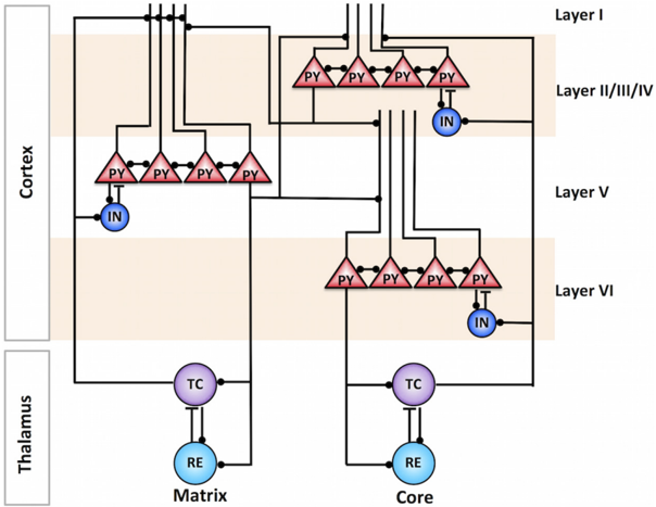
Figure 1 Thalamocortical network model. The cortical column was modeled in three layers: layer II/III/IV, layer V, and layer VI. Each cortical layer was organized in a one-dimensional chain of PY cells and INs. The thalamus model consisted of core and matrix subsystems, including TC and RE neurons. The core TC neurons projected to the middle layers of the cortex (layer II/III/IV), whereas the matrix TC neurons projected to the superficial layer (layer I), making connections to the distal dendrites of layer V pyramidal neurons. The matrix thalamocortical pathway had diffuse connections to the cortex. Black filled circles and black bars represent excitatory and inhibitory connections between neurons, respectively.
Figure 1 Thalamocortical network model. The cortical column was modeled in three layers: layer II/III/IV, layer V, and layer VI. Each cortical layer was organized in a one-dimensional chain of PY cells and INs. The thalamus model consisted of core and matrix subsystems, including TC and RE neurons. The core TC neurons projected to the middle layers of the cortex (layer II/III/IV), whereas the matrix TC neurons projected to the superficial layer (layer I), making connections to the distal dendrites of layer V pyramidal neurons. The matrix thalamocortical pathway had diffuse connections to the cortex. Black filled circles and black bars represent excitatory and inhibitory connections between neurons, respectively.CC-BY-NC-SA · From the PDF
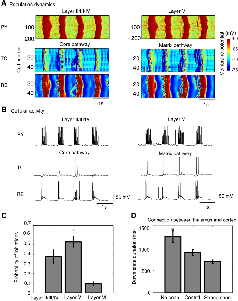
Figure 2 Characteristic properties of slow oscillation in the model. A , Space-time plot representing characteristic activity of the network. The value of the membrane potential for each neuron is indicated with the color code. B , Voltage traces of individual neurons (PY in the layer II/III/IV and layer V, TC and RE in the core and matrix networks). C , Probability of Up-state initiation in three cortical layers. Layer V had higher probability to initiate an Up state. * p < 0.01, one-way ANOVA with Bonferroni's post hoc test. D , Effect of thalamocortical connectivity on slow oscillation. Down-state duration is shown in the model with different connection strength between thalamus and cortex. Increasing connection strength led to significant reduction of Down-state duration. * p < 0.01, one-way ANOVA with Bonferroni's post hoc test. Error bars in C and D indicate STD.
Figure 2 Characteristic properties of slow oscillation in the model. A , Space-time plot representing characteristic activity of the network. The value of the membrane potential for each neuron is indicated with the color code. B , Voltage traces of individual neurons (PY in the layer II/III/IV and layer V, TC and RE in the core and matrix networks). C , Probability of Up-state initiation in three cortical layers. Layer V had higher probability to initiate an Up state. * p < 0.01, one-way ANOVA with Bonferroni's post hoc test. D , Effect of thalamocortical connectivity on slow oscillation. Down-state duration is shown in the model with different connection strength between thalamus and cortex. Increasing connection strength led to significant reduction of Down-state duration. * p < 0.01, one-way ANOVA with Bonferroni's post hoc test. Error bars in C and D indicate STD.CC-BY-NC-SA · From the PDF
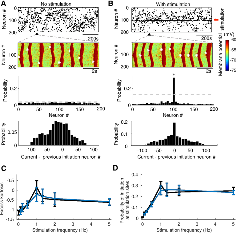
Figure 3 External stimulation influences the spatiotemporal pattern of cortical slow oscillation. A , Representative examples of spontaneous network activity without external input. Top, Up-state initiation sites over the entire simulation time are indicated by black dots. The black triangular indicates the time interval expanded below. Top middle, Characteristic example of the network dynamics. Membrane voltage of pyramidal neurons in layer II/III/IV is indicated with a color code; white stars indicate site of Up-state initiation. Bottom middle, Probability of Up-state initiation across neurons. The dotted line represents mean ± 2 STDs. Bottom, Probability of Up-state initiation at the following cycle ( i + 1) of oscillation as a function of the distance from the initiation site at the previous cycle ( i ). Because of the refractoriness properties of the network, probability of the next active state initiation was higher at the same network site that initiated activity at the previous cycle. B , Periodic (1 Hz) external stimulation (red arrow) was applied to pyramidal cells 101-103 in layer II/III/IV. Same panel description as in A . Note that Up-state initiation occurred mainly near the stimulation site (top). Spatiotemporal pattern of slow-wave propagation became organized (top middle). Probability of Up-state initiation around stimulation sites was increased significantly (bottom middle, * p < 0.01). Excess kurtosis of the Up-state initiation distribution ( C ) and probability of initiation at the simulation sites ( D ) averaged over five different random network initializations as a function of stimulation frequency for Poisson (blue) and periodic (black) stimulation. Two-way ANOVA test showed that there was a significant difference among stimulation frequencies ( p = 3.87 × 10 -12 and p = 1.09 × 10 -24 for C and D , respectively) and no significant difference between Poisson and periodic distributed inputs ( p = 0.8909 and 0.5733 for C and D , respectively). Error bars in C and D indicate STD.
Figure 3 External stimulation influences the spatiotemporal pattern of cortical slow oscillation. A , Representative examples of spontaneous network activity without external input. Top, Up-state initiation sites over the entire simulation time are indicated by black dots. The black triangular indicates the time interval expanded below. Top middle, Characteristic example of the network dynamics. Membrane voltage of pyramidal neurons in layer II/III/IV is indicated with a color code; white stars indicate site of Up-state initiation. Bottom middle, Probability of Up-state initiation across neurons. The dotted line represents mean ± 2 STDs. Bottom, Probability of Up-state initiation at the following cycle ( i + 1) of oscillation as a function of the distance from the initiation site at the previous cycle ( i ). Because of the refractoriness properties of the network, probability of the next active state initiation was higher at the same network site that initiated activity at the previous cycle. B , Periodic (1 Hz) external stimulation (red arrow) was applied to pyramidal cells 101-103 in layer II/III/IV. Same panel description as in A . Note that Up-state initiation occurred mainly near the stimulation site (top). Spatiotemporal pattern of slow-wave propagation became organized (top middle). Probability of Up-state initiation around stimulation sites was increased significantly (bottom middle, * p < 0.01). Excess kurtosis of the Up-state initiation distribution ( C ) and probability of initiation at the simulation sites ( D ) averaged over five different random network initializations as a function of stimulation frequency for Poisson (blue) and periodic (black) stimulation. Two-way ANOVA test showed that there was a significant difference among stimulation frequencies ( p = 3.87 × 10 -12 and p = 1.09 × 10 -24 for C and D , respectively) and no significant difference between Poisson and periodic distributed inputs ( p = 0.8909 and 0.5733 for C and D , respectively). Error bars in C and D indicate STD.CC-BY-NC-SA · From the PDF
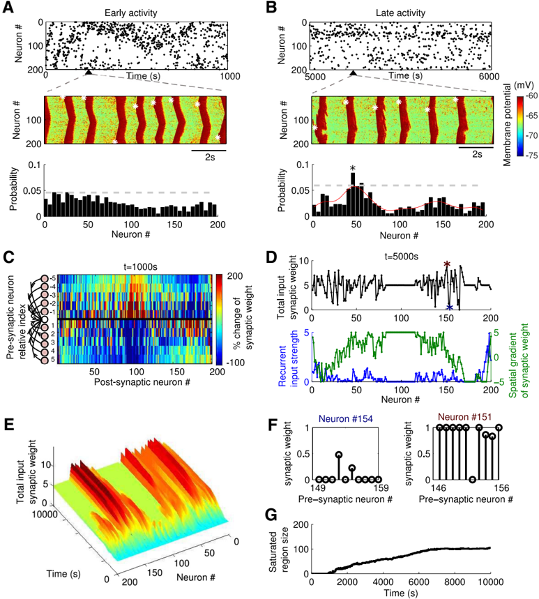
Figure 4 Spontaneous slow oscillation in the presence of STDP. A , B , Representative examples of the network activity during early ( A ) and late ( B ) stages of simulation. Top, Up-state initiation sites are indicated by black dots. The black triangular indicates the time interval expanded below. Middle, Characteristic example of the network dynamics. Membrane voltage of pyramidal neurons in layer II/III/IV is indicated with a color code; white stars indicate the site of Up-state initiation. Bottom, Probability of Up-state initiation across neurons. The dotted line represents mean ± 2STDs. The red curve represents the smoothed histogram by Gaussian filter. Synaptic reorganization leads to appearance of the local groups of neurons preferentially initiating Up states (near cells 50 and 150) during the late stage of simulation (* p < 0.01). C , The percentage change of synaptic weights at time t = 1000 s compared with the initial ( t = 0) synaptic weights shows increase (red) or decrease (blue) of synaptic weights. The x -axis gives the index of the postsynaptic neuron; the y -axis represents the left ( -) and right ( + ) 10 presynaptic neurons relative to the postsynaptic neurons at x -axis. D , At t = 5000 s, total input synaptic weight received by each neuron (top) and recurrent input strength and spatial gradient of synaptic weights (bottom). Note the group of neurons in the middle (neurons 80 -120) with strongly asymmetric connectivity matrix (with connections from one direction of the network enhanced while the connections from the opposite direction reduced) that had high absolute amplitude of spatial gradient would have low probability to initiate the Up states. E , Time evolution of the total (net) input synaptic weight per neuron for 200 pyramidal neurons from layer II/III/IV. F , Individual synaptic weights of two neurons (indicated by stars in D ) with low (left) and high (right) net synaptic weight. G , Time evolution of the size (neuron count) of the cell population that had strongly asymmetric connectivity matrix.
Figure 4 Spontaneous slow oscillation in the presence of STDP. A , B , Representative examples of the network activity during early ( A ) and late ( B ) stages of simulation. Top, Up-state initiation sites are indicated by black dots. The black triangular indicates the time interval expanded below. Middle, Characteristic example of the network dynamics. Membrane voltage of pyramidal neurons in layer II/III/IV is indicated with a color code; white stars indicate the site of Up-state initiation. Bottom, Probability of Up-state initiation across neurons. The dotted line represents mean ± 2STDs. The red curve represents the smoothed histogram by Gaussian filter. Synaptic reorganization leads to appearance of the local groups of neurons preferentially initiating Up states (near cells 50 and 150) during the late stage of simulation (* p < 0.01). C , The percentage change of synaptic weights at time t = 1000 s compared with the initial ( t = 0) synaptic weights shows increase (red) or decrease (blue) of synaptic weights. The x -axis gives the index of the postsynaptic neuron; the y -axis represents the left ( -) and right ( + ) 10 presynaptic neurons relative to the postsynaptic neurons at x -axis. D , At t = 5000 s, total input synaptic weight received by each neuron (top) and recurrent input strength and spatial gradient of synaptic weights (bottom). Note the group of neurons in the middle (neurons 80 -120) with strongly asymmetric connectivity matrix (with connections from one direction of the network enhanced while the connections from the opposite direction reduced) that had high absolute amplitude of spatial gradient would have low probability to initiate the Up states. E , Time evolution of the total (net) input synaptic weight per neuron for 200 pyramidal neurons from layer II/III/IV. F , Individual synaptic weights of two neurons (indicated by stars in D ) with low (left) and high (right) net synaptic weight. G , Time evolution of the size (neuron count) of the cell population that had strongly asymmetric connectivity matrix.CC-BY-NC-SA · From the PDF
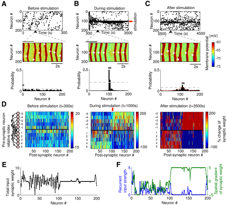
Figure 5 Pattern of slow oscillation in the presence of STDP and external stimulation. A-C , Representative examples of network activity before stimulation ( A ), during stimulation ( B ), and after stimulation ( C ). The site of stimulation is indicated with red arrow. Top, Up-state initiation sites are indicated by black dots. Middle, Characteristic example of the network dynamics. Membrane voltage of pyramidal neurons in layer II/III/IV is indicated with a color code; white stars indicate site of Up-state initiation. Bottom, Probability of Up-state initiation across neurons. The dotted line represents mean ± 2 STDs. The red curve represents the smoothed histogram by Gaussian filter. Note that the probability of Up-state initiation was very high around the stimulation site (cell 100) during stimulation ( B , * p < 0.01), and it remained high after stimulation was terminated ( C , * p < 0.01). D , The percentage change of synaptic weights at time t = 300s(left), t = 1000s(middle), and t = 3500 s (right) compared with the initial ( t = 0) synaptic weights. The x -axis gives the index of the postsynaptic neuron, and the y -axis represents the left ( -) and right ( + ) 10 presynaptic neurons relative to the postsynaptic neurons at x -axis. E , Total input synaptic weight received by each neuron at the end of stimulation ( t = 3500s). F , Recurrent input strength and spatial gradient of synaptic weight at t = 3500 s.
Figure 5 Pattern of slow oscillation in the presence of STDP and external stimulation. A-C , Representative examples of network activity before stimulation ( A ), during stimulation ( B ), and after stimulation ( C ). The site of stimulation is indicated with red arrow. Top, Up-state initiation sites are indicated by black dots. Middle, Characteristic example of the network dynamics. Membrane voltage of pyramidal neurons in layer II/III/IV is indicated with a color code; white stars indicate site of Up-state initiation. Bottom, Probability of Up-state initiation across neurons. The dotted line represents mean ± 2 STDs. The red curve represents the smoothed histogram by Gaussian filter. Note that the probability of Up-state initiation was very high around the stimulation site (cell 100) during stimulation ( B , * p < 0.01), and it remained high after stimulation was terminated ( C , * p < 0.01). D , The percentage change of synaptic weights at time t = 300s(left), t = 1000s(middle), and t = 3500 s (right) compared with the initial ( t = 0) synaptic weights. The x -axis gives the index of the postsynaptic neuron, and the y -axis represents the left ( -) and right ( + ) 10 presynaptic neurons relative to the postsynaptic neurons at x -axis. E , Total input synaptic weight received by each neuron at the end of stimulation ( t = 3500s). F , Recurrent input strength and spatial gradient of synaptic weight at t = 3500 s.CC-BY-NC-SA · From the PDF
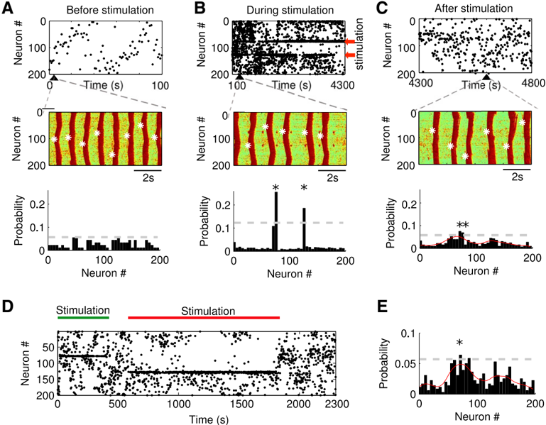
Image 6
CC-BY-NC-SA · From the PDF
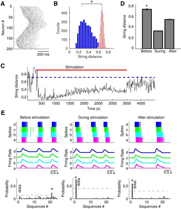
Figure 7 Spike sequence replay. A , Spike raster plot of a typical Up state. B , Distribution of the SDs between every sequence and all the other sequences from the subset of Up states initiated at thesamenetworklocation,repeatedindependentlyforeachnetworklocation(blue),anddistributionofSDsbetweeneverysequenceandalltheothersequenceswithrandomlyshuffledspiketimes from the same subset of Up states, repeated independently for each network location (red). There was a significant difference between the means of the two distributions (* p < 0.01, MannWhitney U test). C , SD between template sequence (sequence 101, 102, 100, 103, 99, 104, 98 … for initiation site 101) and spike sequences from all the Up states as a function of time. Stimulation was applied at sites 101-103; red bar indicates stimulation time. Blue dotted line represents mean SD between the template sequence and sequences extracted from Up states before stimulation. D , Mean SD between a template spike sequence and all the spike sequences before, during (from 300 to 3500 s, red bar), and after stimulation, as shown in C . Mean SDs during and after stimulation weresignificantly different from that before stimulation (* p < 0.01, one-way ANOVA with Bonferroni's post hoc test). Error bars indicate standard error. E , Representative examples of four neurons (a = 20, b = 35, c = 50, d = 65) spike trains (top), smoothed firing rate (middle), and probability of each sequence (bottom) before, during, and after stimulation. The dotted line represents mean ± 2 STDs. Note the high probability of the 'dcba' sequence during (* p < 0.01) and after (* p < 0.01) stimulation.
Figure 7 Spike sequence replay. A , Spike raster plot of a typical Up state. B , Distribution of the SDs between every sequence and all the other sequences from the subset of Up states initiated at thesamenetworklocation,repeatedindependentlyforeachnetworklocation(blue),anddistributionofSDsbetweeneverysequenceandalltheothersequenceswithrandomlyshuffledspiketimes from the same subset of Up states, repeated independently for each network location (red). There was a significant difference between the means of the two distributions (* p < 0.01, MannWhitney U test). C , SD between template sequence (sequence 101, 102, 100, 103, 99, 104, 98 … for initiation site 101) and spike sequences from all the Up states as a function of time. Stimulation was applied at sites 101-103; red bar indicates stimulation time. Blue dotted line represents mean SD between the template sequence and sequences extracted from Up states before stimulation. D , Mean SD between a template spike sequence and all the spike sequences before, during (from 300 to 3500 s, red bar), and after stimulation, as shown in C . Mean SDs during and after stimulation weresignificantly different from that before stimulation (* p < 0.01, one-way ANOVA with Bonferroni's post hoc test). Error bars indicate standard error. E , Representative examples of four neurons (a = 20, b = 35, c = 50, d = 65) spike trains (top), smoothed firing rate (middle), and probability of each sequence (bottom) before, during, and after stimulation. The dotted line represents mean ± 2 STDs. Note the high probability of the 'dcba' sequence during (* p < 0.01) and after (* p < 0.01) stimulation.CC-BY-NC-SA · From the PDF
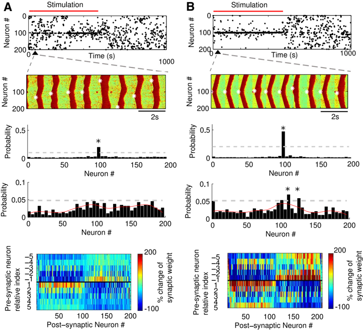
Figure 8 Effect of global network stimulation. Local input (at neurons 101, 102, 103) was applied without ( A ) and simultaneously with ( B ) global modulation of the network activity. Top, Up-state initiation sites (black dots). Red bar represents the time of stimulation. Top middle, Representative example of spatiotemporal patterns of Up and Down states. Note the higher synchrony of slow oscillation in the presence of global stimulation (right). Middle, Distribution of Up-state initiation sites during the entire 1000 s simulation time. Bottom middle, Distribution of Up-state initiation sites after stimulation. Bottom, The percentage change of synaptic weights at the end of stimulation ( t = 500 s) compared with initial ( t = 0) synaptic weights. The x -axis gives the index of the postsynaptic neuron, and the y -axis represents the left ( -) and right ( + ) presynaptic neurons relative to the postsynaptic neurons at the x -axis. The dotted line represents mean ± 2 STDs, whereas * p < 0.01 from z score. The red curve represents the smoothed histogram by Gaussian filter.
Figure 8 Effect of global network stimulation. Local input (at neurons 101, 102, 103) was applied without ( A ) and simultaneously with ( B ) global modulation of the network activity. Top, Up-state initiation sites (black dots). Red bar represents the time of stimulation. Top middle, Representative example of spatiotemporal patterns of Up and Down states. Note the higher synchrony of slow oscillation in the presence of global stimulation (right). Middle, Distribution of Up-state initiation sites during the entire 1000 s simulation time. Bottom middle, Distribution of Up-state initiation sites after stimulation. Bottom, The percentage change of synaptic weights at the end of stimulation ( t = 500 s) compared with initial ( t = 0) synaptic weights. The x -axis gives the index of the postsynaptic neuron, and the y -axis represents the left ( -) and right ( + ) presynaptic neurons relative to the postsynaptic neurons at the x -axis. The dotted line represents mean ± 2 STDs, whereas * p < 0.01 from z score. The red curve represents the smoothed histogram by Gaussian filter.CC-BY-NC-SA · From the PDF

Verification

Claims the paper makes

The claims and statistics of this paper haven’t been checked yet.

Run the check — free, no account needed. It reads the open-access text and checks the sources it cites.

A few free checks a day · papers already verified open instantly · results are public

Claims other papers make about this one

Each is checked against this paper’s own text: does it say what the citing paper says it does?

Self-check

Percentages, sums and reported differences re-computed from the paper’s own numbers.

The self-check needs the paper’s full text.

Citations

Cites

Show all 67 references

Cited by

Sorted by citations

Items 101–116 of 116

Metadata

Authors
Wei, Y., Krishnan, G. P., & Bazhenov, M.
Affiliations
University of California, Riverside (US)
Venue
The Journal of Neuroscience
Published
2016-04-13
Volume
36
Issue
15
Pages
4231-4247
ISSN
  • 0270-6474 (ISSN-L)
  • 1529-2401
OpenAlex
W2340922036
Cited by
116
References
67
Citations by year
2026: 8 · 2025: 7 · 2024: 8 · 2023: 28 · 2022: 15 · 2021: 9 · 2020: 13 · 2019: 8 · 2018: 9 · 2017: 8 · 2016: 3
FWCI
5.94
Type
journal article
Language
en
Open access
Locations
  • Journal of Neuroscience (publishedVersion, cc-by-nc-sa)
  • PubMed Central (publishedVersion)
  • PubMed (publishedVersion)
Funders
  • National Institutes of Health (MH099645)
  • Multidisciplinary University Research Initiative
  • Office of Naval Research (N00014-13-1-0672, R01 EB009282, R01 MH099645)
  • National Institute of Mental Health (R01MH099645)
  • National Institute of Biomedical Imaging and Bioengineering (R01EB009282)
Topics
  • Life Sciences › Neuroscience › Cognitive Neuroscience › Sleep and Wakefulness Research
  • Life Sciences › Neuroscience › Cognitive Neuroscience › Neural dynamics and brain function
  • Life Sciences › Neuroscience › Cognitive Neuroscience › Memory and Neural Mechanisms
Keywords
memory consolidation, slow oscillations, slow-wave sleep, synaptic plasticity, spike-timing-dependent plasticity, thalamocortical network, hippocampal ripples, sharp-wave ripples, computational model
MeSH terms
Algorithms, Cerebral Cortex, Computer Simulation, Electroencephalography, Humans, Memory, Models, Neurological, Neuronal Plasticity, Neurons, Sleep, Synapses, Thalamus, Calcium Channels, Sodium Channels, Neural Networks, Computer

About these checks

Registry, retraction, Cites and statistics results are computed, not judged, with one exception: a printed reference that no index lists is read once by a model before it counts as a citation error. Claims are extracted by a model and kept only when their quote appears verbatim in the text; each cited source is then checked, with a model’s help, for whether it says what the claim relies on. Those verdicts can be wrong — read the claim’s quote and the cited source before relying on one.

Statistics and arithmetic are recomputed, not judged.

Confidence bands are shown only for fields calibrated on our annotated test set. None is calibrated yet, so no band is shown.

What counts as a claim ›How we measure confidence ›How we check this ›

Are you an author, or do you see a problem with this page? Request a review