PreprintCited by 31Transcranial Magnetic Stimulation StudiesStroke Rehabilitation and RecoveryDeep Brain Stimulation and Movement Disorders

The DOI matches its Crossref record; 1 of the 1 references it cites were found in a registry or an index.

Deep Cerebellar Transcranial Direct Current Stimulation of the Dentate Nucleus to Facilitate Standing Balance in Chronic Stroke Survivors

Open access

Preprint — published as 10.3390/brainsci10020094 · Paper page

Abstract

Objective: Cerebrovascular accidents are the second leading cause of death and the third leading cause of disability worldwide. We hypothesized that cerebellar transcranial direct current stimulation (ctDCS) of the dentate nuclei and the lower-limb representations in the cerebellum can improve standing balance functional reach in chronic (> 6 months’ post-stroke) stroke survivors. Materials and Methods: Magnetic resonance imaging(MRI) based subject-specific electric field was computed across 10 stroke survivors and one healthy MRI template to find an optimal bipolar bilateral ctDCS montage to target dentate nuclei and lower-limb representations (lobules VII-IX). Then, in a repeated-measure crossover study on 5 stroke survivors, we compared 15minutes of 2mA ctDCS based on the effects on successful functional reach(%) during standing balance task. Three-way ANOVA investigated the factors of interest– brain regions, montages, stroke participants, and their interactions.Results: “One-size-fits-all” ctDCS montage for the clinical study was found to be bipolar PO9h – PO10h for dentate nuclei and bipolar Exx7–Exx8 for lobules VII-IX with contalesional anode. Bipolar PO9h–PO10h ctDCS performed significantly (alpha=0.05) better in facilitating successful functional reach (%) when compared to bipolar Exx7–Exx8 ctDCS. Furthermore, a linear relationship between successful functional reach (%) and electric field strength was found where bipolar PO9h–PO10h montage resulted in a significantly (alpha=0.05) higher electric field strength when compared to bipolar Exx7–Exx8 montage for the same 2mA current. Conclusion: We presented a rational neuroimaging based approach to optimize deep ctDCS of the dentate nuclei and lower limb representations in the cerebellum for post-stroke balance rehabilitation.

Overview

The claims and statistics of this paper haven’t been checked yet.

Run the check — free, no account needed. It reads the open-access text and checks the sources it cites.

A few free checks a day · papers already verified open instantly · results are public

Integrity signals

Registry

Crossref · 10.20944/preprints201912.0235.v1

Cites

1 of 1 references verified0 citation errors · 0 not checkable

Statistics

Figures

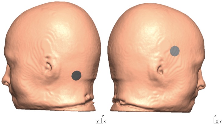
Figure A1 The head model from the 55–59 years old MRI template is shown below with two tentative electrode locations and the X, Y, and the Z-direction of the global coordinate system.
Figure A1 The head model from the 55–59 years old MRI template is shown below with two tentative electrode locations and the X, Y, and the Z-direction of the global coordinate system.CC BY · PubMed Central
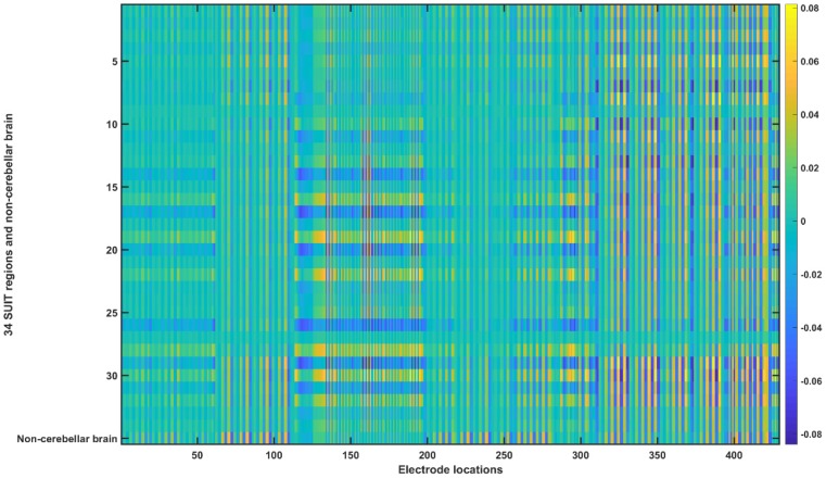
Figure A2 Ex transfer matrix for the head model from the 55–59 years old MRI template. The X-axis shows the electrode locations (refer Appendix B) and Y-axis shows the 34 SUIT regions (refer Appendix A) and non-cerebellar brain.
Figure A2 Ex transfer matrix for the head model from the 55–59 years old MRI template. The X-axis shows the electrode locations (refer Appendix B) and Y-axis shows the 34 SUIT regions (refer Appendix A) and non-cerebellar brain.CC BY · PubMed Central
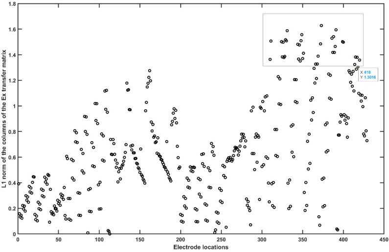
Figure A3 L1 norm of the columns of the Ex transfer matrix without the non-cerebellar brain (i.e. row 35). The rectangle shows the electrode locations with the high L1 norm (electrodes relevant for cerebellar stimulation in Ex).
Figure A3 L1 norm of the columns of the Ex transfer matrix without the non-cerebellar brain (i.e. row 35). The rectangle shows the electrode locations with the high L1 norm (electrodes relevant for cerebellar stimulation in Ex).CC BY · PubMed Central
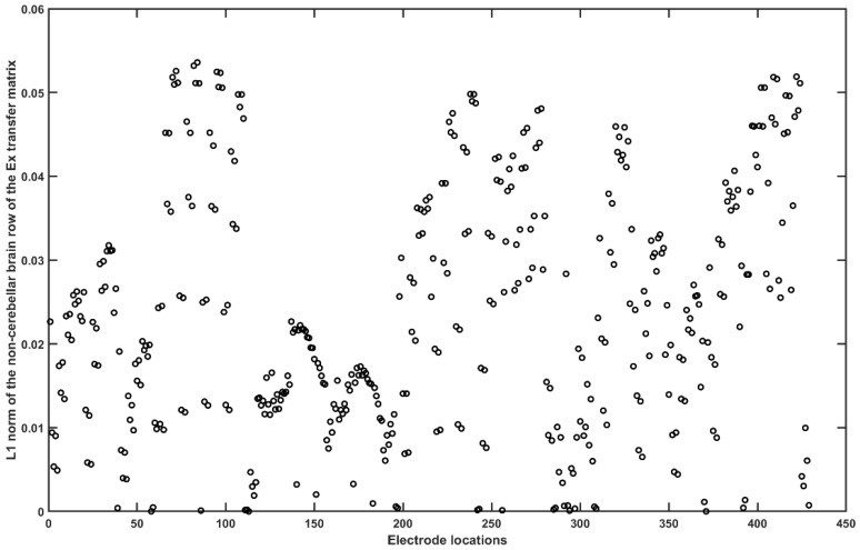
Figure A4 L1 norm of the non-cerebellar brain row (= 35) of the Ex transfer matrix.
Figure A4 L1 norm of the non-cerebellar brain row (= 35) of the Ex transfer matrix.CC BY · PubMed Central
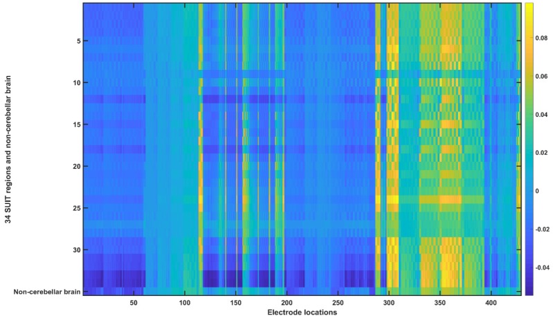
Figure A5 Ey transfer matrix for the head model from the 55–59 years old MRI template. The X-axis shows the electrode locations (refer Appendix B) and Y-axis shows the 34 SUIT regions (refer Appendix A) and non-cerebellar brain.
Figure A5 Ey transfer matrix for the head model from the 55–59 years old MRI template. The X-axis shows the electrode locations (refer Appendix B) and Y-axis shows the 34 SUIT regions (refer Appendix A) and non-cerebellar brain.CC BY · PubMed Central
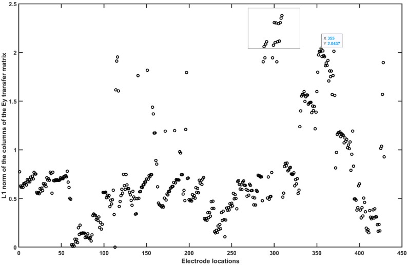
Figure A6 L1 norm of the columns of the Ey transfer matrix without the non-cerebellar brain (i.e. row 35). The rectangle shows the electrode locations with the high L1 norm (electrodes relevant for cerebellar stimulation in Ey).
Figure A6 L1 norm of the columns of the Ey transfer matrix without the non-cerebellar brain (i.e. row 35). The rectangle shows the electrode locations with the high L1 norm (electrodes relevant for cerebellar stimulation in Ey).CC BY · PubMed Central
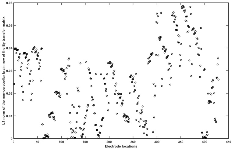
Figure A7 L1 norm of the non-cerebellar brain row (= 35) of the Ey transfer matrix.
Figure A7 L1 norm of the non-cerebellar brain row (= 35) of the Ey transfer matrix.CC BY · PubMed Central
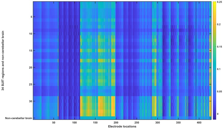
Figure A8 Ez transfer matrix for the head model from the 55–59 years old MRI template. The X-axis shows the electrode locations (refer Appendix B) and Y-axis shows the 34 SUIT regions (refer Appendix A) and non-cerebellar brain.
Figure A8 Ez transfer matrix for the head model from the 55–59 years old MRI template. The X-axis shows the electrode locations (refer Appendix B) and Y-axis shows the 34 SUIT regions (refer Appendix A) and non-cerebellar brain.CC BY · PubMed Central
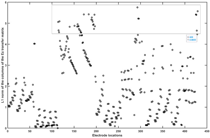
Figure A9 L1 norm of the columns of the Ez transfer matrix without the non-cerebellar brain (i.e., row 35). The rectangle shows the electrode locations with the high L1 norm (electrodes relevant for cerebellar stimulation in Ez).
Figure A9 L1 norm of the columns of the Ez transfer matrix without the non-cerebellar brain (i.e., row 35). The rectangle shows the electrode locations with the high L1 norm (electrodes relevant for cerebellar stimulation in Ez).CC BY · PubMed Central
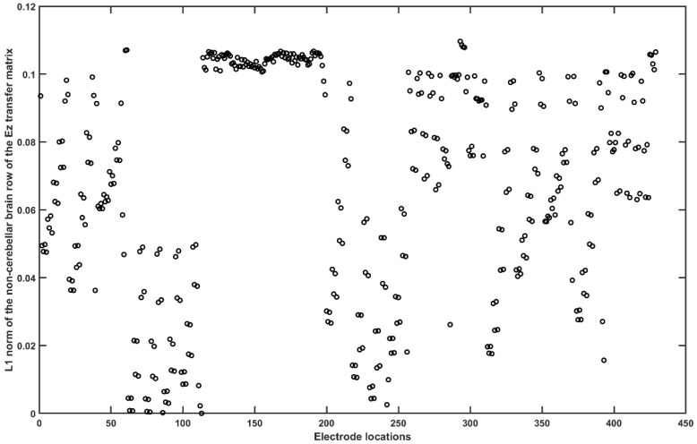
Figure A10 L1 norm of the non-cerebellar brain row (= 35) of the Ez transfer matrix.
Figure A10 L1 norm of the non-cerebellar brain row (= 35) of the Ez transfer matrix.CC BY · PubMed Central
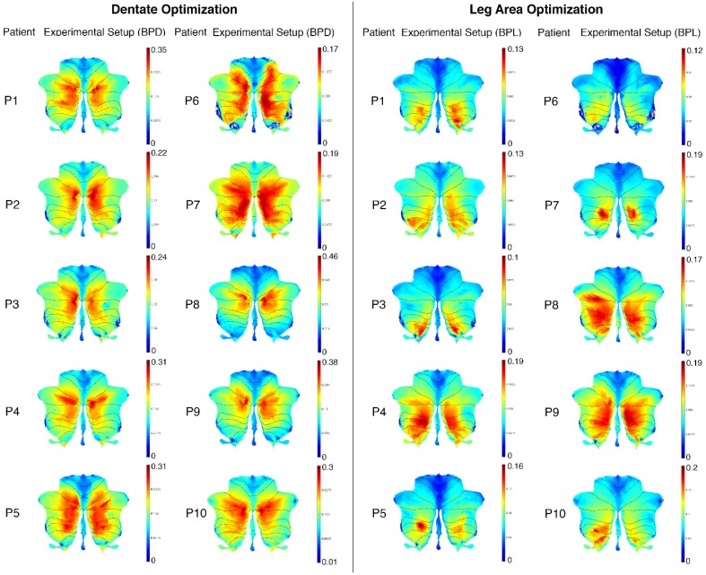
Figure A11 Post-stroke subject-specific SUIT flatmaps for all the 10 participants.
Figure A11 Post-stroke subject-specific SUIT flatmaps for all the 10 participants.CC BY · PubMed Central
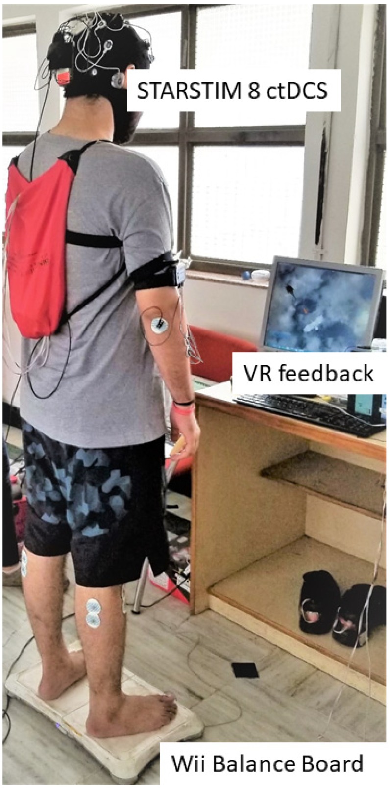
Figure 1 Portable experimental setup for the clinical study consisting of the Wii Balance Board to measure the center of pressure (CoP), a small form factor desktop PC with monitor for the virtual reality (VR) balance testing and training based on CoP. And the wireless STARSTIM 8 simulator for cerebellar transcranial direct current stimulation (ctDCS).
Figure 1 Portable experimental setup for the clinical study consisting of the Wii Balance Board to measure the center of pressure (CoP), a small form factor desktop PC with monitor for the virtual reality (VR) balance testing and training based on CoP. And the wireless STARSTIM 8 simulator for cerebellar transcranial direct current stimulation (ctDCS).CC BY · PubMed Central
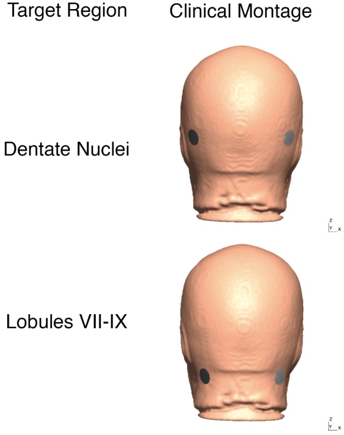
Figure 2 Clinical bilateral ctDCS montages used for FRT balance study is shown on the head model from 55 to 59 years age-group MRI template. Top panel: bipolar at PO9h-PO10h, Bottom panel: bipolar at Exx7–Exx8.
Figure 2 Clinical bilateral ctDCS montages used for FRT balance study is shown on the head model from 55 to 59 years age-group MRI template. Top panel: bipolar at PO9h-PO10h, Bottom panel: bipolar at Exx7–Exx8.CC BY · PubMed Central
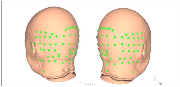
Figure 3 Reduced set of 87 electrode locations to optimize bipolar ctDCS montage for stroke survivors, namely: “E145”, “E146”, “E156”, “E165”, “Ex1”, “Ex2”, “Ex3”, “Ex4”, “Ex5”, “Ex6”, “Ex7”, “Ex8”, “Exx10”, “Exx11”, “Exx12”, “Exx1”, “Exx2”, “Exx3”, “Exx4”, “Exx5”, “Exx6”, “Exx7”, “Exx8”, “Exx9”, “Exxz”, “Exz”, “I1h”, “I2h”, “Iz”, “NkB”, “NkL”, “NkR”, “O1”, “O1h”, “O2”, “O2h”, “OI1”, “OI1h”, “OI2”, “OI2h”, “OIz”, “Oz”, “P10”, “P10h”, “P7”, “P7h”, “P8”, “P8h”, “P9”, “P9h”, “PO10”, “PO10h”, “PO7”, “PO7h”, “PO8”, “PO8h”, "PO9”, “PO9h”, “POO10”, “POO10h”, “POO1h”, “POO2”, “POO2h”, “POO3h”, “POO8”, “POO9”, “POO9h”, “POOz”, “PPO10”, “PPO10h”, “PPO7”, “PPO7h”, “PPO8”, “PPO8h”, “PPO9”, “PPO9h”, “T5”, “T6”, “TPP10h”, “TPP7”, “TPP8”, “TPP8h”, “TPP9h”, “Z1”, “Z2”, “Z7”, “Z9”. The global coordinate system shown by colored vectors, red: X, green: Y, blue: Z.
Figure 3 Reduced set of 87 electrode locations to optimize bipolar ctDCS montage for stroke survivors, namely: “E145”, “E146”, “E156”, “E165”, “Ex1”, “Ex2”, “Ex3”, “Ex4”, “Ex5”, “Ex6”, “Ex7”, “Ex8”, “Exx10”, “Exx11”, “Exx12”, “Exx1”, “Exx2”, “Exx3”, “Exx4”, “Exx5”, “Exx6”, “Exx7”, “Exx8”, “Exx9”, “Exxz”, “Exz”, “I1h”, “I2h”, “Iz”, “NkB”, “NkL”, “NkR”, “O1”, “O1h”, “O2”, “O2h”, “OI1”, “OI1h”, “OI2”, “OI2h”, “OIz”, “Oz”, “P10”, “P10h”, “P7”, “P7h”, “P8”, “P8h”, “P9”, “P9h”, “PO10”, “PO10h”, “PO7”, “PO7h”, “PO8”, “PO8h”, "PO9”, “PO9h”, “POO10”, “POO10h”, “POO1h”, “POO2”, “POO2h”, “POO3h”, “POO8”, “POO9”, “POO9h”, “POOz”, “PPO10”, “PPO10h”, “PPO7”, “PPO7h”, “PPO8”, “PPO8h”, “PPO9”, “PPO9h”, “T5”, “T6”, “TPP10h”, “TPP7”, “TPP8”, “TPP8h”, “TPP9h”, “Z1”, “Z2”, “Z7”, “Z9”. The global coordinate system shown by colored vectors, red: X, green: Y, blue: Z.CC BY · PubMed Central
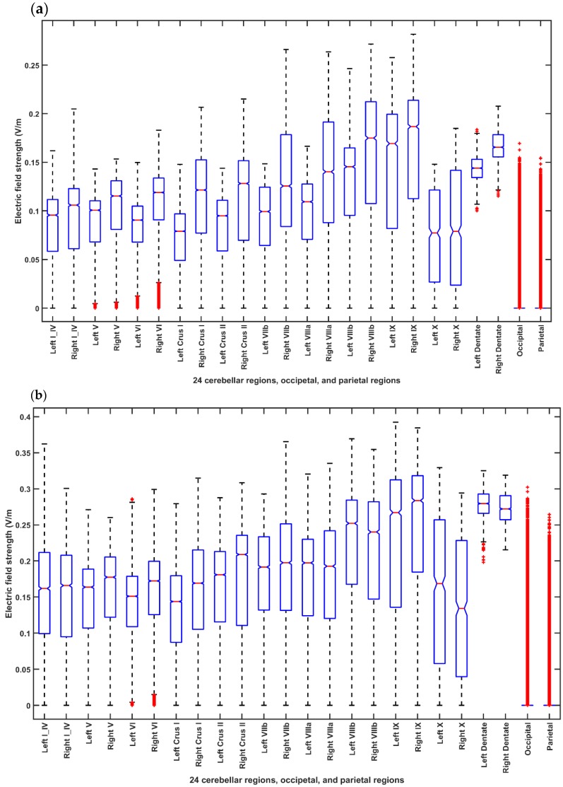
Figure 4 Boxplot of the electric field distribution for different ctDCS montages for the head model from the MRI template of 55-59 years age-group across 24 cerebellar regions, occipital and parietal lobes where in each box, the central mark indicates the median, and the bottom and top edges of the box indicate the 25th and 75th percentiles, respectively. The whiskers extend to the most extreme data points not considered outliers, and the outliers are plotted individually using the ‘+’ symbol. If the notches in the box plot do not overlap, one can conclude, with 95% confidence that the true medians do differ. (a) Shows the EF distribution for the Celnik montage. (b) Shows the EF distribution for the Manto montage. (c) Shows the EF distribution for the Extracephalic montage. (d) Shows the EF distribution for the PO9h–PO10h montage for case 1 (Optimization for dentate nucleus). (e) Shows the EF distribution for the Exx7–Exx8 montage for case 2 (Optimization for lobules VII–IX). (f) ANOVA table: Two-way ANOVA for the factors of interest–montages (X1), brain regions (X2), and their interactions (montage* brain region)–all found significant. Source: Source of variability; Sum Sq.: Sum of Squares due to each source; d. f.: Degrees of freedom associated with each source; Mean Sq.: Mean Square for each source, which is the ratio Sum Sq. /d. f. F: statistics which is the ratio of the mean squares.
Figure 4 Boxplot of the electric field distribution for different ctDCS montages for the head model from the MRI template of 55-59 years age-group across 24 cerebellar regions, occipital and parietal lobes where in each box, the central mark indicates the median, and the bottom and top edges of the box indicate the 25th and 75th percentiles, respectively. The whiskers extend to the most extreme data points not considered outliers, and the outliers are plotted individually using the ‘+’ symbol. If the notches in the box plot do not overlap, one can conclude, with 95% confidence that the true medians do differ. (a) Shows the EF distribution for the Celnik montage. (b) Shows the EF distribution for the Manto montage. (c) Shows the EF distribution for the Extracephalic montage. (d) Shows the EF distribution for the PO9h–PO10h montage for case 1 (Optimization for dentate nucleus). (e) Shows the EF distribution for the Exx7–Exx8 montage for case 2 (Optimization for lobules VII–IX). (f) ANOVA table: Two-way ANOVA for the factors of interest–montages (X1), brain regions (X2), and their interactions (montage* brain region)–all found significant. Source: Source of variability; Sum Sq.: Sum of Squares due to each source; d. f.: Degrees of freedom associated with each source; Mean Sq.: Mean Square for each source, which is the ratio Sum Sq. /d. f. F: statistics which is the ratio of the mean squares.CC BY · PubMed Central
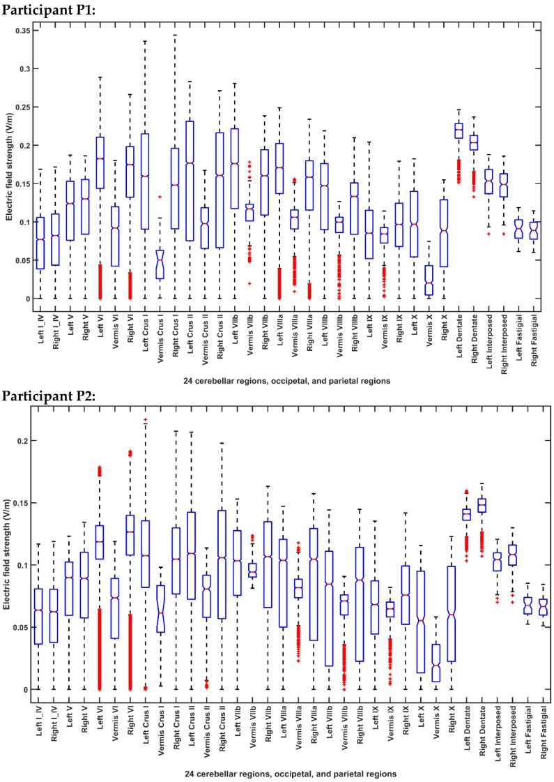
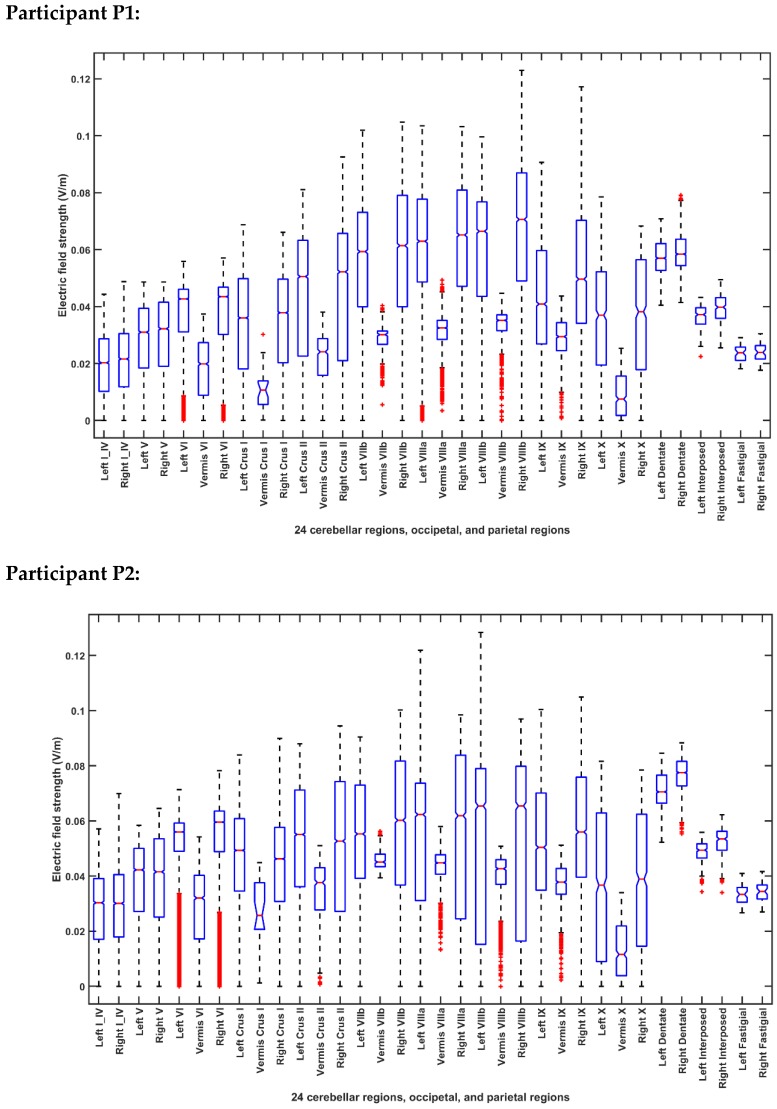
Figure 5 Boxplot of the lobular electric field distribution for the 10 post-stroke patients for the PO9h–PO10h montage for case 1 (optimization for dentate nuclei).
Figure 5 Boxplot of the lobular electric field distribution for the 10 post-stroke patients for the PO9h–PO10h montage for case 1 (optimization for dentate nuclei).CC BY · PubMed Central
Figure 6 Boxplot of the lobular electric field distribution for the 10 post-stroke patients for the Exx7–Exx8 montage for case 2 (optimization for bilateral lobules VII–IX).
Figure 6 Boxplot of the lobular electric field distribution for the 10 post-stroke patients for the Exx7–Exx8 montage for case 2 (optimization for bilateral lobules VII–IX).CC BY · PubMed Central
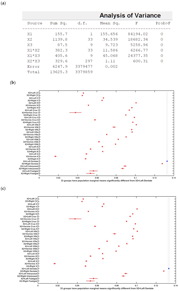
Figure 7 (a) ANOVA table: Three-way ANOVA for the factors of interest–montages (X1), brain regions (X2), subject (X3), and their interactions–all found significant. (b) Results of the multiple comparison test of the population marginal means between the PO9h–PO10h montage and the Exx7 – Exx8 montage (X1). (c) Results of the multiple comparison test of the population marginal means of different brain regions (X2). The dentate nuclei were exposed to the highest electric field strength (>0.12 V/m) across montages (X1) and subjects (X3). (d) Results of the multiple comparison test of the population marginal means of different subjects (X3). Subject P8 was exposed to the highest electric field strength (>0.1 V/m) across montages (X1) and brain regions (X2). Source: Source of variability;.Sum Sq.: Sum of Squares due to each source; d. f.: Degrees of freedom associated with each source; Mean Sq.: Mean Square for each source, which is the ratio Sum Sq. /d. f. F: statistics which is the ratio of the mean squares.
Figure 7 (a) ANOVA table: Three-way ANOVA for the factors of interest–montages (X1), brain regions (X2), subject (X3), and their interactions–all found significant. (b) Results of the multiple comparison test of the population marginal means between the PO9h–PO10h montage and the Exx7 – Exx8 montage (X1). (c) Results of the multiple comparison test of the population marginal means of different brain regions (X2). The dentate nuclei were exposed to the highest electric field strength (>0.12 V/m) across montages (X1) and subjects (X3). (d) Results of the multiple comparison test of the population marginal means of different subjects (X3). Subject P8 was exposed to the highest electric field strength (>0.1 V/m) across montages (X1) and brain regions (X2). Source: Source of variability;.Sum Sq.: Sum of Squares due to each source; d. f.: Degrees of freedom associated with each source; Mean Sq.: Mean Square for each source, which is the ratio Sum Sq. /d. f. F: statistics which is the ratio of the mean squares.CC BY · PubMed Central
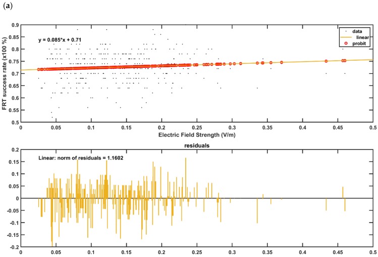
Figure 8 (a,b) GLM model (with probit link) for the post-intervention FRT success rate (%) with the lobular maximum electric field strength as the predictor in (a), and with the lobular median electric field strength as the predictor in the (b). The plot shows the observed and estimated the FRT success rate (%) versus the predictor values as well as the residuals where the FRT success rate (%) found to be more sensitive to lobular median electric field strength (slope 0.17—Figure 8b) than the lobular maximum electric field strength (slope 0.09—Figure 8a). (c,d) GLM model (with probit link) for the post-intervention FRT success rate (%) with the median electric field strength in dentate nuclei as the predictor in the c), and with the median electric field strength in the bilateral cerebellar leg area lobules as the predictor in the (d). The plot shows the observed and estimated the FRT success rate (%) versus the predictor values as well as the residuals where the FRT success rate (%) found to be more sensitive to the leg area lobular median electric field strength (slope 0.34—Figure 8d) than the dentate nuclei median electric field strength (slope 0.27—Figure 8c).
Figure 8 (a,b) GLM model (with probit link) for the post-intervention FRT success rate (%) with the lobular maximum electric field strength as the predictor in (a), and with the lobular median electric field strength as the predictor in the (b). The plot shows the observed and estimated the FRT success rate (%) versus the predictor values as well as the residuals where the FRT success rate (%) found to be more sensitive to lobular median electric field strength (slope 0.17—Figure 8b) than the lobular maximum electric field strength (slope 0.09—Figure 8a). (c,d) GLM model (with probit link) for the post-intervention FRT success rate (%) with the median electric field strength in dentate nuclei as the predictor in the c), and with the median electric field strength in the bilateral cerebellar leg area lobules as the predictor in the (d). The plot shows the observed and estimated the FRT success rate (%) versus the predictor values as well as the residuals where the FRT success rate (%) found to be more sensitive to the leg area lobular median electric field strength (slope 0.34—Figure 8d) than the dentate nuclei median electric field strength (slope 0.27—Figure 8c).CC BY · PubMed Central

Verification

Claims the paper makes

The claims and statistics of this paper haven’t been checked yet.

Run the check — free, no account needed. It reads the open-access text and checks the sources it cites.

A few free checks a day · papers already verified open instantly · results are public

Self-check

Percentages, sums and reported differences re-computed from the paper’s own numbers.

The self-check needs the paper’s full text.

Citations

Cites

Show all 1 references

Metadata

Authors
Rezaee, Z., Kaura, S., Solanki, D., Dash, A., Srivastava, M. V. P., Lahiri, U., & Dutta, A.
Affiliations
  • University at Buffalo, State University of New York (US)
  • All India Institute of Medical Sciences (IN)
  • Indian Institute of Technology Gandhinagar (IN)
Corresponding author
Dutta, Anirban
Venue
Brain Sciences
Publisher
MDPI AG
Published
2019-12-18
Volume
10
Issue
2
Pages
94-94
ISSN
2076-3425 (ISSN-L)
OpenAlex
W2994623943
Cited by
31
References
1
Citations by year
2026: 2 · 2025: 2 · 2024: 4 · 2023: 5 · 2022: 9 · 2021: 8 · 2020: 1
FWCI
2.21
Type
journal article
Language
en
Open access
Locations
  • Brain Sciences (publishedVersion, cc-by)
  • Preprints.org (acceptedVersion, cc-by)
  • PubMed Central (publishedVersion, cc-by)
  • PubMed (publishedVersion)
  • DOAJ (DOAJ: Directory of Open Access Journals) (submittedVersion, cc-by-sa)
Funders
  • Institut national de recherche en informatique et en automatique (INRIA)
  • Department of Science and Technology, Ministry of Science and Technology, India
  • Ministry of Education, India
  • Scheme for Promotion of Academic and Research Collaboration
  • Division of Human Resource Development
Topics
  • Life Sciences › Neuroscience › Neurology › Transcranial Magnetic Stimulation Studies
  • Health Sciences › Medicine › Rehabilitation › Stroke Rehabilitation and Recovery
  • Health Sciences › Medicine › Clinical Neurology › Deep Brain Stimulation and Movement Disorders
Keywords
transcranial direct current stimulation, dentate nucleus, cerebellum, chronic stroke, standing balance, postural control, functional reach test, stroke rehabilitation

About these checks

Registry, retraction, Cites and statistics results are computed, not judged, with one exception: a printed reference that no index lists is read once by a model before it counts as a citation error. Claims are extracted by a model and kept only when their quote appears verbatim in the text; each cited source is then checked, with a model’s help, for whether it says what the claim relies on. Those verdicts can be wrong — read the claim’s quote and the cited source before relying on one.

Statistics and arithmetic are recomputed, not judged.

Confidence bands are shown only for fields calibrated on our annotated test set. None is calibrated yet, so no band is shown.

What counts as a claim ›How we measure confidence ›How we check this ›

Are you an author, or do you see a problem with this page? Request a review

How to cite

Cite CoChat for the checks on this page, and the paper for its own findings.

This page
CoChat. (2026). Citation check: Deep Cerebellar Transcranial Direct Current Stimulation of the Dentate Nucleus to Facilitate Standing Balance in Chronic Stroke Survivors. https://app.cochat.ai/papers/10.20944/preprints201912.0235.v1
The paper
Rezaee, Z., Kaura, S., Solanki, D., Dash, A., Srivastava, M. V. P., Lahiri, U., & Dutta, A. (2019). Deep Cerebellar Transcranial Direct Current Stimulation of the Dentate Nucleus to Facilitate Standing Balance in Chronic Stroke Survivors. Brain Sciences. https://doi.org/10.20944/preprints201912.0235.v1