

The DOI matches its Crossref record; 88 of the 90 references it cites were found in a registry or an index; none of the 54 sources its claims cite is checked for support yet.
Thickness Characteristics of Pāhoehoe Lavas in the Deccan Province, Western Ghats, India, and in Continental Flood Basalt Provinces Elsewhere
Open accessAbstract
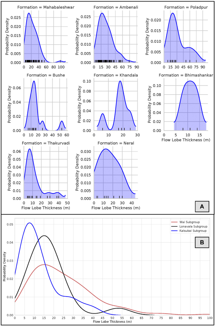
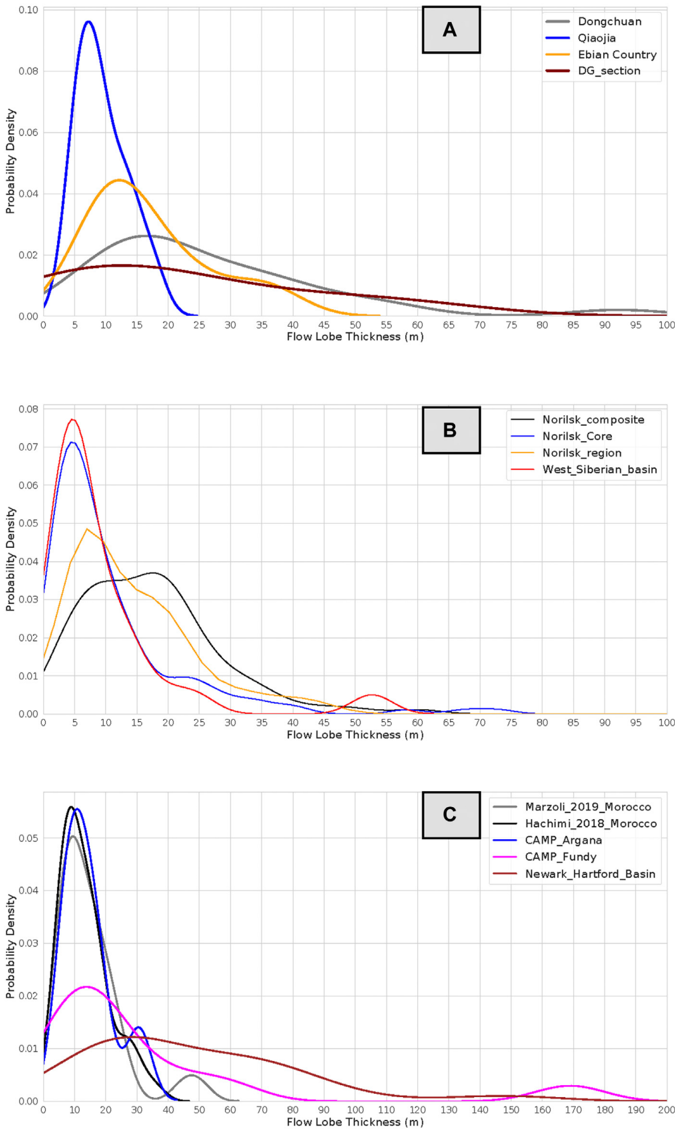
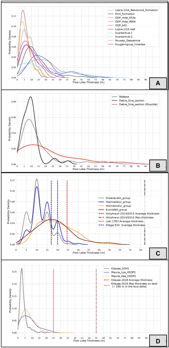
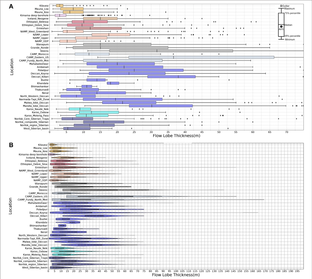
Constraining the eruption rates of flood basalt lava flows remains a significant challenge despite decades of work. One potential observable proxy for eruption rates is flood basalt lava-flow lobe thicknesses, a topic that we tackle here quantitatively. In this study, we provide the first global compilation of pāhoehoe lava-lobe thicknesses from various continental flood basalt provinces (∼ 3,800 measurements) to compare characteristic thicknesses within and between provinces. We refer to thin lobes (∼ ≤5 m), characteristic of “compound” lavas, as hummocky pāhoehoe lava flows or flow-fields. Conversely, we term thicker lobes, characteristic of “simple” flows, as coming from sheet-lobe-dominated flows. Data from the Deccan Traps and Columbia River flood-basalt provinces are archetypal since they have the most consistent datasets as well as established chemo- and litho-stratigraphies. Examining Deccan lobe thicknesses, we find that previously suggested (and disputed) distinct temporal and regional distributions of hummocky pāhoehoe and sheet-lobe-dominated flow fields are not strongly supported by the data and that each geochemically defined formation displays both lobe types in varying amounts. Thin flow-lobes do not appear to indicate proximity to source. The modal lobe thickness of Deccan formations with abundant “thin” lava-lobes is 8 m, while the mode for sheet-lobe-dominated formations is only 17 m. Sheet-lobes up to 75–80 m are rare in the Deccan and Columbia River Provinces, and ones >100 m are exceptional globally. For other flood basalt provinces, modal thickness plots show a prevalence toward similar lobe thicknesses to Deccan, with many provinces having some or most lobes in the 5–8 m modal range. However, median values are generally thicker, in the 8–12 m range, suggesting that sheet-lobes dominate. By contrast, lobes from non-flood basalt flow-fields (e.g., Hawai’i, Snake River Plain) show distinctly thinner modes, sub-5 m. Our results provide a quantitative basis to ascertain variations in gross lava morphology and, perhaps, this will in future be related to emplacement dynamics of different flood basalt provinces, or parts thereof. We can also systematically distinguish outlier lobes (or regions) from typical lobes in a province, e.g., North American Central Atlantic Magmatic Province lava-lobes are anomalously thick and are closely related to feeder-intrusions, thus enabling a better understanding of conditions required to produce large-volume, thick, flood basalt lava-lobes and flows.
Overview
CoChat Summary
Written by AI from the paper’s full text.
TL;DR
This paper compiles ~3,800 pāhoehoe lava-lobe thickness measurements to compare continental flood basalt provinces, focusing on the Deccan Traps. It finds that CFB sheet-lobes typically cluster around 15–20 m globally, while non-flood-basalt systems such as Hawai‘i and the Snake River Plain have distinctly thinner modes.
Key findings
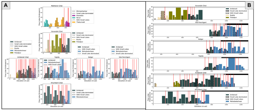
- In the Deccan, formations with abundant thin lava-lobes have a modal lobe thickness of 8 m, while sheet-lobe-dominated formations have a mode of 17 m; sheet-lobes up to 75–80 m are rare, and >100 m lobes are exceptional globally.
- The global mode for pāhoehoe sheet-lobes in CFB provinces is 15–20 m; many provinces have modes in the 5–8 m range, but median values are generally 8–12 m, suggesting sheet-lobe dominance.
- Non-flood-basalt flow-fields show thinner modes: Hawai‘i and Snake River Plain modal lobe thicknesses are 3–7 m, with Kīlauea at 3 m and Mauna Loa/Mauna Kea at 8 m.
- Hummocky pāhoehoe flow-fields represent approximately 5% of the total thickness of the Deccan Wai Subgroup but up to 77% in some Kalsubai Subgroup formations, based on one traverse.
Methods
- The study compiles ~3,800 individual lava-lobe thickness measurements from continental flood basalt provinces and modern analogs, with primary datasets from the Deccan, Columbia River Basalt, and Karoo provinces.
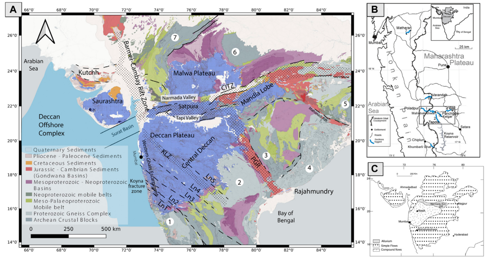
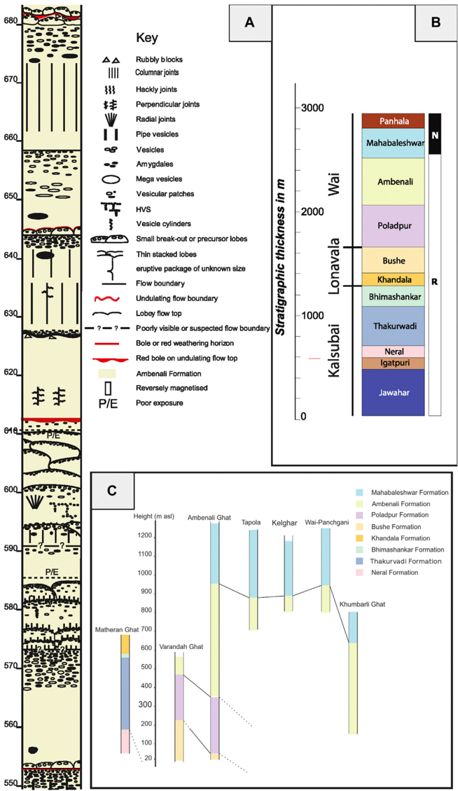
- Deccan data come from detailed volcanological logs covering ~5 km of lava flows across multiple transects, plus drill cores from Koyna and Killari and previously published sections from other Deccan subprovinces.
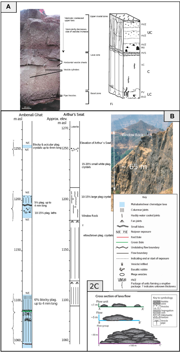
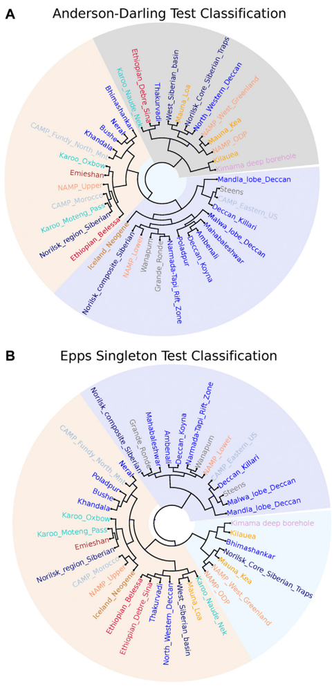
- Lobe thickness was measured from the top of the upper crust to the bottom of the lower crust; thin lobes (<2 m) were measured by tape (±~10 cm), thicker lobes by barometric altimeter with differential GPS anchoring. Data are analyzed using kernel density estimators, violin plots, and Anderson-Darling and Epps-Singleton tests with hierarchical clustering.
Limitations
- The paper states that small lobes are likely under-reported, the thickest lobes are rarely completely exposed, and the thinnest lobes are too numerous and/or weathered to measure accurately, so both size extremes are underrepresented.
- It also states that only one Deccan traverse includes the lowest Kalsubai Subgroup formations, that Deccan data come from a small region of the central Western Ghats and may have regional bias, and that other CFB datasets are more variable in quantity and quality.
- The text notes that a maximum reported Koyna core lobe thickness of 165 m must be treated with suspicion, that some datasets may be locationally biased, and that all reported data are from syn- and post-Mesozoic lavas; the relationship between lobe thickness and eruption rates remains an open question.
Model-written summary. Check it against the paper before relying on it.
Integrity signals
Registry
Cites
Statistics
Figures
Verification
Claims the paper makes
61 Own result · 26 Own interpretation · 23 Own method · 20 No full text of the sources · 12 Check pending · 8 Not checked yet · 4 Sources not found · 4 No basis given
A result the paper reports from its own data — it cites no other source for it, so there is none to check. The quote shows it is in the paper.
In the paper
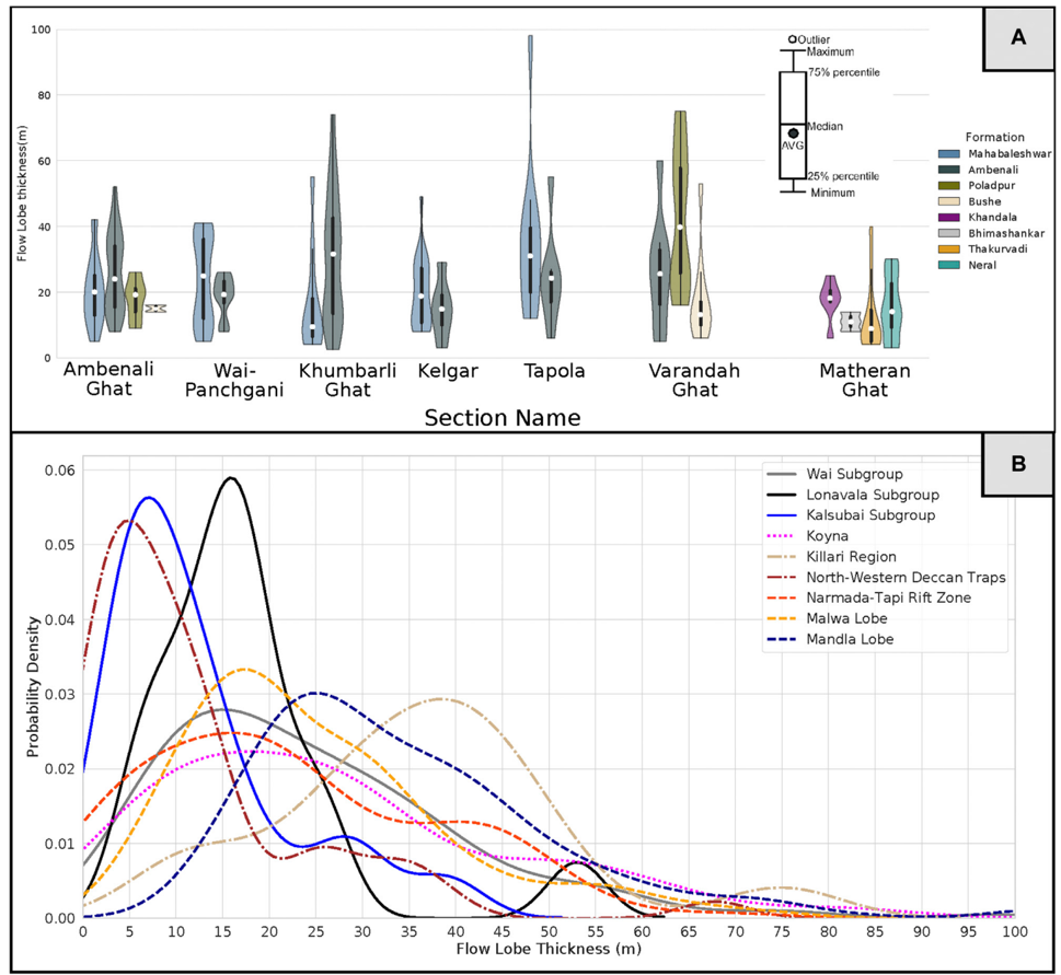
“The flows in this region are most like the Wai Subgroup flows in terms of their thickness distributions.”
§ Thickness Characteristics of P ahoehoe Lavas in the Deccan Province, Western Ghats, India, and in Continental Flood Basalt Provinces Elsewhere > Deccan Volcanic Province Including Koyna Region
plainstates an association- Asserted: passes — The authors put it forward as true.
- Checkable: passes — It can be checked against evidence.
- Load-bearing: passes — The paper’s conclusions depend on it.
- Based: passes — The paper gives a reason why it holds.
A result the paper reports from its own data — it cites no other source for it, so there is none to check. The quote shows it is in the paper.
In the paper
“The plot clearly shows that the thickest SLs are in the minority in terms of occurrence.”
§ Thickness Characteristics of P ahoehoe Lavas in the Deccan Province, Western Ghats, India, and in Continental Flood Basalt Provinces Elsewhere > Deccan Volcanic Province Including Koyna Region
boosted- Asserted: passes — The authors put it forward as true.
- Checkable: passes — It can be checked against evidence.
- Load-bearing: unclear — It is unclear whether the paper’s conclusions depend on it.
- Based: passes — The paper gives a reason why it holds.
A result the paper reports from its own data — it cites no other source for it, so there is none to check. The quote shows it is in the paper.
In the paper
“By contrast, the flows in the north-western Deccan (Saurashtra region) are similar to the oldest Western Ghats flows (Kalsubai group) in terms of lobe thickness (Figure 6B).”
§ Thickness Characteristics of P ahoehoe Lavas in the Deccan Province, Western Ghats, India, and in Continental Flood Basalt Provinces Elsewhere > Deccan Volcanic Province Including Koyna Region
plain- Asserted: passes — The authors put it forward as true.
- Checkable: passes — It can be checked against evidence.
- Load-bearing: unclear — It is unclear whether the paper’s conclusions depend on it.
- Based: passes — The paper gives a reason why it holds.
In the paper
“No strong pattern of variation is evident, yet southward could be more distal from some suggested sources areas (Vanderkluysen et al., 2011).”
§ Thickness Characteristics of P ahoehoe Lavas in the Deccan Province, Western Ghats, India, and in Continental Flood Basalt Provinces Elsewhere > Deccan Volcanic Province Including Koyna Region
What the sources say
- Not checked — no full text of the sourcecites Vanderkluysen et al., 2011 source
hedged- Asserted: passes — The authors put it forward as true.
- Checkable: passes — It can be checked against evidence.
- Load-bearing: passes — The paper’s conclusions depend on it.
- Based: passes — The paper gives a reason why it holds.
A result the paper states — it cites no source for it, so there is none to check. The quote shows it is in the paper.
In the paper
“and ones >100 m are exceptional globally.”
§ Thickness Characteristics of P ahoehoe Lavas in the Deccan Province, Western Ghats, India, and in Continental Flood Basalt Provinces Elsewhere > Abstract
plain- Asserted: passes — The authors put it forward as true.
- Checkable: passes — It can be checked against evidence.
- Load-bearing: passes — The paper’s conclusions depend on it.
- Based: passes — The paper gives a reason why it holds.
- It may state two separate claims as one. 55
- Probably not a substantial claim. 29
Create a free account to see these claims.
Create a free account to see these assumptions.
80 more claims
Create a free account to see all 158 claims and to verify the 15 references still open.
Self-check
Percentages, sums and reported differences re-computed from the paper’s own numbers.
Each contradiction between two passages listed here was confirmed by an independent check.
Rated major: it would touch a result — a value a result rests on, reported and recomputed p-values on opposite sides of the significance level, two passages that conflict with no sign which is right, or a cited work retracted before this paper was published.
In the paper
§ Thickness Characteristics of P ahoehoe Lavas in the Deccan Province, Western Ghats, India, and in Continental Flood Basalt Provinces Elsewhere > Deccan Volcanic Province Including Koyna Region
“The thickest SLs are generally in the range 50-60 m for the Wai Sub-group and Bushe Formation lavas”
§ Thickness Characteristics of P ahoehoe Lavas in the Deccan Province, Western Ghats, India, and in Continental Flood Basalt Provinces Elsewhere > Characteristics of Deccan Volcanic Province Lavas
“the Bushe Formation, which has a similar lobe-size distribution to the Wai lavas except for lacking lobes >∼ 20 m thick”
Rated minor: it would not touch a result — a value no result rests on, a p-value that stays on the same side of the significance level, or a conflict that is clerical, resolved elsewhere in the paper, or outside its own findings.
In the paper
§ Thickness Characteristics of P ahoehoe Lavas in the Deccan Province, Western Ghats, India, and in Continental Flood Basalt Provinces Elsewhere > Abstract
“By contrast, lobes from non-flood basalt flow-fields (e.g., Hawai'i, Snake River Plain) show distinctly thinner modes, sub-5 m.”
§ Thickness Characteristics of P ahoehoe Lavas in the Deccan Province, Western Ghats, India, and in Continental Flood Basalt Provinces Elsewhere > Other CFB Provinces and Hawai'i
“The modal lobe thickness is 8 m for the two large shield volcanoes, contrasting strongly with that of K ilauea.”
Citations
Cites
SciPy 1.0: fundamental algorithms for scientific computing in Python
Virtanen, P., Gommers, R., Oliphant, T. E., Haberland, M., Reddy, T., Cournapeau, D., Burovski, E., Peterson, P., Weckesser, W., Bright, J., et al. (2020) · Nature Methods · doi:10.1038/s41592-019-0686-2 · Cited by 38,430
ETE 3: Reconstruction, Analysis, and Visualization of Phylogenomic Data
Huerta‐Cepas, J., Serra, F., & Bork, P. (2016) · Molecular Biology and Evolution · doi:10.1093/molbev/msw046 · Cited by 2,255
Atmospheric and environmental effects of the 1783–1784 Laki eruption: A review and reassessment
Thordarson, T., & Self, S. (2003) · Journal of Geophysical Research Atmospheres · doi:10.1029/2001jd002042 · Cited by 602
Self-citationU-Pb constraints on pulsed eruption of the Deccan Traps across the end-Cretaceous mass extinction
Schoene, B., Eddy, M. P., Samperton, K. M., Keller, C. B., Keller, G., Adatte, T., & Khadri, S. F. R. (2019) · Science · doi:10.1126/science.aau2422 · Cited by 542
K-Sample Anderson–Darling Tests
Scholz, F., & Stephens, M. A. (1987) · Journal of the American Statistical Association · doi:10.1080/01621459.1987.10478517 · Cited by 532
State shift in Deccan volcanism at the Cretaceous-Paleogene boundary, possibly induced by impact
Renne, P. R., Sprain, C. J., Richards, M. A., Self, S., Vanderkluysen, L., & Pande, K. (2015) · Science · doi:10.1126/science.aac7549 · Cited by 431
Self-citationThe eruptive tempo of Deccan volcanism in relation to the Cretaceous-Paleogene boundary
Sprain, C. J., Renne, P. R., Vanderkluysen, L., Pande, K., Self, S., & Mittal, T. (2019) · Science · doi:10.1126/science.aav1446 · Cited by 395
Self-citationStratigraphy, composition and form of the Deccan Basalts, Western Ghats, India
Beane, J. E., Turner, C. A., Hooper, P. R., Subbarao, K. V., & Walsh, J. N. (1986) · Bulletin of Volcanology · doi:10.1007/bf01073513 · Cited by 384
Self, S., Keszthelyi, L. P., & Thordarson, T. (1998) · Annual Review of Earth and Planetary Sciences · doi:10.1146/annurev.earth.26.1.81 · Cited by 382
Self-citationCompound and simple lava flows and flood basalts
Walker, G. P. L. (1971) · Bulletin Volcanologique · doi:10.1007/bf02596829 · Cited by 306
Research works printed but not linked: 13
- Deshmukh, 1988, Petrographic variations in compound flows of Deccan Traps and their significance, 305
- Garcia, 2007, Stratigraphy of the Hawai’i Scientific Drilling Project core (HSDP2): anatomy of a Hawai’ian shield volcano, Geochem. Geophys. Geosyst., 8, 1525, 10.1016/j.jvolgeores.2019.07.007 · DOI · Paper page
- Godbole, 1996, Lava stratigraphy of Deccan Basalts of Western Maharashtra, 125
- Guilbaud, 2005, Morphology, surface structures, and emplacement of lavas produced by Laki, AD 1783–1784, Geol. Soc. America Spec. Pap., 396, 81, 10.1130/2005.2396(07 · DOI
- Gupta, 2003, Borehole investigations in the surface rupture zone of the 1993 Latur SCR earthquake, Maharashtra, India: overview of results, 1
- Kasiviswanandham, 2003, Flow stratigraphy and paleomagnetic investigations of Bagli Volcanics, Malwa Deccan Traps MP, and to develop constraints on its petrogenesis
- Puffer, 1992, The palisades sill and Watchung Basalt flows, Northern New Jersey and Southeastern New York: a geological summary and field guide, 92
- Raja Rao, 1999, Distribution, structure and petrography of the Deccan Traps, India, 401
- Self, 1997, Emplacement of continental flood Basalt lava flows, 381
- Sharma, 2000, Variations in cooling, crystallization textures, and glass chemistry during emplacement of Kilauea Pahoehoe lobes, as constrained by in situ field experiments, GSA Abstr. Programs, 32
- K. V., 1999, Deccan volcanic province, 547
- Swanson, Chronological narrative of the 1969-71 Mauna Ulu eruption of Kilauea volcano, Hawaii, U.S.
- Walker, 1999, Some observations and interpretations on the Deccan Traps, 367
Cited by
The life cycle of large igneous provinces
Black, B. A., Karlstrom, L., & Mather, T. A. (2021) · Nature Reviews Earth & Environment · doi:10.1038/s43017-021-00221-4 · Cited by 102
The Magmatic Architecture of Continental Flood Basalts I: Observations From the Deccan Traps
Mittal, T., Richards, M. A., & Fendley, I. M. (2021) · Journal of Geophysical Research: Solid Earth · doi:10.1029/2021jb021808 · Cited by 42
Self-citationToward Understanding Deccan Volcanism
Self, S., Mittal, T., Vanderkluysen, L., & Dole, G. (2022) · Annual Review of Earth and Planetary Sciences · doi:10.1146/annurev-earth-012721-051416 · Cited by 37
Self-citationThe Magmatic Architecture of Continental Flood Basalts: 2. A New Conceptual Model
Mittal, T., & Richards, M. A. (2021) · Journal of Geophysical Research: Solid Earth · doi:10.1029/2021jb021807 · Cited by 16
Self-citationDiverse Lava Flow Morphologies in the Stratigraphy of the Jezero Crater Floor
Alwmark, S., Horgan, B. H. N., Udry, A., Bechtold, A., Fagents, S. A., Ravanis, E. M., Crumpler, L. S., Schmitz, N., Cloutis, E. A., Brown, A. J., et al. (2023) · Journal of Geophysical Research Planets · doi:10.1029/2022je007446 · Cited by 25
Metadata
- Authors
- Self, S., Mittal, T., & Jay, A. E.
- Affiliations
- University of California, Berkeley (US)
- Massachusetts Institute of Technology (US)
- The Open University (GB)
- Corresponding author
- Self, Stephen
- Venue
- Frontiers in Earth Science
- Publisher
- Frontiers Media SA
- Published
- 2021-02-17
- Volume
- 8
- ISSN
- 2296-6463 (ISSN-L)
- OpenAlex
- W3038594804
- Cited by
- 33
- References
- 90
- Citations by year
- 2026: 2 · 2025: 8 · 2024: 6 · 2023: 5 · 2022: 5 · 2021: 7
- FWCI
- 3.09
- Type
- journal article
- Language
- en
- Open access
- gold
- doi.org
- Licence
- Locations
- Frontiers in Earth Science (publishedVersion, cc-by)
- Open Research Online (The Open University) (acceptedVersion)
- DSpace@MIT (Massachusetts Institute of Technology) (submittedVersion, cc-by)
- DOAJ (DOAJ: Directory of Open Access Journals) (submittedVersion, cc-by-sa)
- Funders
- National Science Foundation
- Topics
- Physical Sciences › Earth and Planetary Sciences › Geochemistry and Petrology › Geological and Geochemical Analysis
- Physical Sciences › Earth and Planetary Sciences › Geology › Geological and Geophysical Studies
- Physical Sciences › Earth and Planetary Sciences › Earth-Surface Processes › Geological formations and processes
- Keywords
- pahoehoe lava, continental flood basalts, Deccan Traps, Columbia River Basalt Group, eruption rate, lava flow morphology, flood basalt province
About these checks
Registry, retraction, Cites and statistics results are computed, not judged, with one exception: a printed reference that no index lists is read once by a model before it counts as a citation error. Claims are extracted by a model and kept only when their quote appears verbatim in the text; each cited source is then checked, with a model’s help, for whether it says what the claim relies on. Those verdicts can be wrong — read the claim’s quote and the cited source before relying on one.
A language model drew the claims from the paper on 2026-11-12, under version 3 of the claim definition (model deepseek-v4.1-flash, prompt extract-v3).
A second model labelled each claim on 2026-11-12 (model jev-1.13-20260917, definition revision gold-guideline-v0.2).
Statistics and arithmetic are recomputed, not judged.
Confidence bands are shown only for fields calibrated on our annotated test set. None is calibrated yet, so no band is shown.
What counts as a claim ›How we measure confidence ›How we check this ›
Are you an author, or do you see a problem with this page? Request a review
