Cited by 361Gut microbiota and healthMicrobial Community Ecology and PhysiologyOral microbiology and periodontitis research

The DOI matches its Crossref record; 71 of the 71 references it cites were found in a registry or an index.

The Power of Microbiome Studies: Some Considerations on Which Alpha and Beta Metrics to Use and How to Report Results

Open access
Kers, Jannigje Gerdien, Saccenti, Edoardo·2022·Frontiers in Microbiology

Published version of a preprint

Abstract

Background: Since sequencing techniques have become less expensive, larger sample sizes are applicable for microbiota studies. The aim of this study is to show how, and to what extent, different diversity metrics and different compositions of the microbiota influence the needed sample size to observe dissimilar groups. Empirical 16S rRNA amplicon sequence data obtained from animal experiments, observational human data, and simulated data were used to perform retrospective power calculations. A wide variation of alpha diversity and beta diversity metrics were used to compare the different microbiota datasets and the effect on the sample size. Results: Our data showed that beta diversity metrics are the most sensitive to observe differences as compared with alpha diversity metrics. The structure of the data influenced which alpha metrics are the most sensitive. Regarding beta diversity, the Bray–Curtis metric is in general the most sensitive to observe differences between groups, resulting in lower sample size and potential publication bias. Conclusion: We recommend performing power calculations and to use multiple diversity metrics as an outcome measure. To improve microbiota studies, awareness needs to be raised on the sensitivity and bias for microbiota research outcomes created by the used metrics rather than biological differences. We have seen that different alpha and beta diversity metrics lead to different study power: because of this, one could be naturally tempted to try all possible metrics until one or more are found that give a statistically significant test result, i.e., p -value < α. This way of proceeding is one of the many forms of the so-called p -value hacking. To this end, in our opinion, the only way to protect ourselves from (the temptation of) p -hacking would be to publish a statistical plan before experiments are initiated, describing the outcomes of interest and the corresponding statistical analyses to be performed.

Overview

The claims and statistics of this paper haven’t been checked yet.

Run the check — free, no account needed. It reads the open-access text and checks the sources it cites.

A few free checks a day · papers already verified open instantly · results are public

Integrity signals

Registry

Crossref · 10.3389/fmicb.2021.796025

Cites

71 of 71 references verified0 citation errors · 0 not checkable

Statistics

Figures

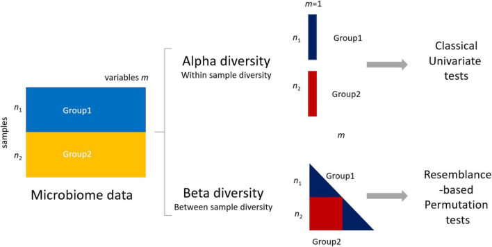
FIGURE 1 Differences between group 1 (data matrix X1 − n1 samples × m1 variables/microbial features) and group 2 in microbiome data can be assessed using either alpha (within-sample diversity) or beta (between-sample diversity) metrics. The use of alpha metrics allows the use of classical univariate testing, either parametric or nonparametric. The use of beta metrics leads to the use of permutation-based testing approaches like permutational multivariate ANOVA (PERMANOVA) (see section “Materials and Methods”).
FIGURE 1 Differences between group 1 (data matrix X1 − n1 samples × m1 variables/microbial features) and group 2 in microbiome data can be assessed using either alpha (within-sample diversity) or beta (between-sample diversity) metrics. The use of alpha metrics allows the use of classical univariate testing, either parametric or nonparametric. The use of beta metrics leads to the use of permutation-based testing approaches like permutational multivariate ANOVA (PERMANOVA) (see section “Materials and Methods”).CC BY · PubMed Central
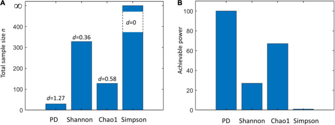
FIGURE 2 (A) Total sample size (n) required to assess the statistical significance of a given effect d using a two-sample Kruskal–Wallis test with a power equal to 0.8 and confidence α = 0.01 when using different alpha metrics (phylogenetic diversity (PD), Shannon’s, Chao1, and Simpson’s indices). (B) Achievable power attainable by a Kruskal–Wallis test using a total sample size n = n1+ n2 = 50 + 50 = 100 using different alpha metrics (same as A). Note that for a null effect (d = 0), the achievable power coincides with α. Effect sizes are calculated from the Human Microbiome Project (HMP) data (comparison of skin and vaginal microbiome) reported in Table 1.
FIGURE 2 (A) Total sample size (n) required to assess the statistical significance of a given effect d using a two-sample Kruskal–Wallis test with a power equal to 0.8 and confidence α = 0.01 when using different alpha metrics (phylogenetic diversity (PD), Shannon’s, Chao1, and Simpson’s indices). (B) Achievable power attainable by a Kruskal–Wallis test using a total sample size n = n1+ n2 = 50 + 50 = 100 using different alpha metrics (same as A). Note that for a null effect (d = 0), the achievable power coincides with α. Effect sizes are calculated from the Human Microbiome Project (HMP) data (comparison of skin and vaginal microbiome) reported in Table 1.CC BY · PubMed Central
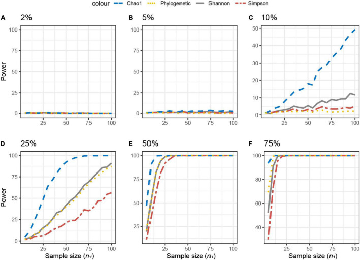
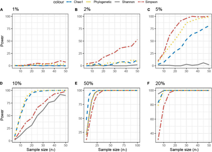
FIGURE 3 Empirical power of a two-sample Kruskal–Wallis test for the univariate comparison of two simulated microbiome datasets X1 and X2 [Simulated dataset 1: this simulation generates data under an exist–non-exist binary scenario where bacterial features are either present or absent in X1 and X2. The data have the same phylogenetic structure of the Human Microbiome Project (HMP) Gut data described in Table 1] using different alpha diversity metrics (phylogenetic, Chao1, Shannon’s, and Simpson’s indices; see Equations 3–6 in section “Materials and Methods”). The empirical power is calculated using Equation (11) as a function of the sample size n1 of group 1 (with n2 = n1 and total sample size n = n1 + n2) using K = 1,000 replications. (A–F) The analysis of data simulations in which 2, 5, 10, 25, 50, and 75% of bacterial features are not present in dataset X2 with respect to X1, respectively.
FIGURE 3 Empirical power of a two-sample Kruskal–Wallis test for the univariate comparison of two simulated microbiome datasets X1 and X2 [Simulated dataset 1: this simulation generates data under an exist–non-exist binary scenario where bacterial features are either present or absent in X1 and X2. The data have the same phylogenetic structure of the Human Microbiome Project (HMP) Gut data described in Table 1] using different alpha diversity metrics (phylogenetic, Chao1, Shannon’s, and Simpson’s indices; see Equations 3–6 in section “Materials and Methods”). The empirical power is calculated using Equation (11) as a function of the sample size n1 of group 1 (with n2 = n1 and total sample size n = n1 + n2) using K = 1,000 replications. (A–F) The analysis of data simulations in which 2, 5, 10, 25, 50, and 75% of bacterial features are not present in dataset X2 with respect to X1, respectively.CC BY · PubMed Central
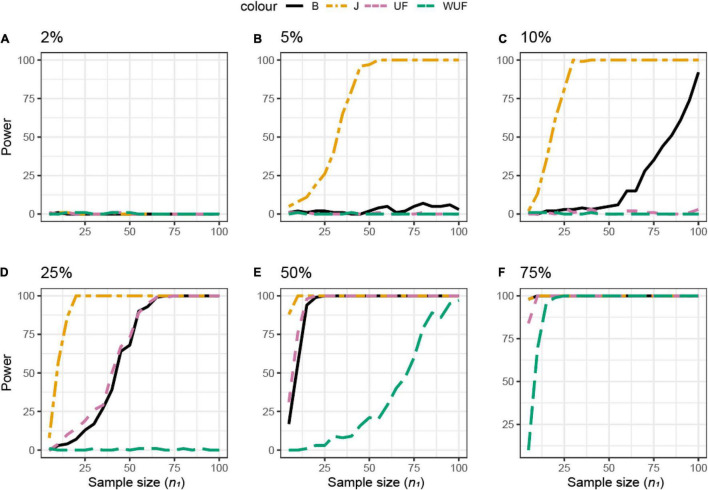
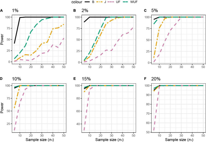
FIGURE 4 Empirical power of a permutational multivariate ANOVA (PERMANOVA) test for the multivariate comparison of two simulated microbiome datasets X1 and X2 [Simulated dataset 1: this simulation generates data under an exist–non-exist binary scenario where bacterial features are either present or absent in X1 and X2. The data have the same phylogenetic structure of the Human Microbiome Project (HMP) Gut data described in Table 1] using different beta diversity metrics [Bray–Curtis dissimilarity (B), Jaccard (J), unweighted UniFrac (UF), and weighted UniFrac (WUF) distances; see Equations (7)–(9), and (6) in section “Materials and Methods”]. The empirical power is calculated using Equation (11) as a function of the sample size n1 of group 1 (with n2 = n1 and total sample size n = n1 + n2) using K = 100 replications. (A–F) The analysis of data simulations in which 2, 5, 10, 25, 50, and 75% of bacterial features are not present in dataset X2 with respect to X1, respectively.
FIGURE 4 Empirical power of a permutational multivariate ANOVA (PERMANOVA) test for the multivariate comparison of two simulated microbiome datasets X1 and X2 [Simulated dataset 1: this simulation generates data under an exist–non-exist binary scenario where bacterial features are either present or absent in X1 and X2. The data have the same phylogenetic structure of the Human Microbiome Project (HMP) Gut data described in Table 1] using different beta diversity metrics [Bray–Curtis dissimilarity (B), Jaccard (J), unweighted UniFrac (UF), and weighted UniFrac (WUF) distances; see Equations (7)–(9), and (6) in section “Materials and Methods”]. The empirical power is calculated using Equation (11) as a function of the sample size n1 of group 1 (with n2 = n1 and total sample size n = n1 + n2) using K = 100 replications. (A–F) The analysis of data simulations in which 2, 5, 10, 25, 50, and 75% of bacterial features are not present in dataset X2 with respect to X1, respectively.CC BY · PubMed Central
FIGURE 5 Empirical power of a two-sample Kruskal–Wallis test for the univariate comparison of two simulated microbiome datasets X1 and X2 [Simulated dataset 2: This simulation thus generates data under a differential abundant scenario where bacterial features are present in the different compositions in X1 and X2. The data have the same phylogenetic structure of the Human Microbiome Project (HMP) Gut data described in Table 1] using different alpha diversity metrics [phylogenetic, Chao1, Shannon’s, and Simpson’s indices; see Equations (3)–(5), and (6) in section “Materials and Methods”]. The empirical power is calculated using Equation (11) as a function of the sample size n1 of group 1 (with n2 = n1 and total sample size n = n1 + n2) using K = 1,000 replications. (A–F) The analysis of data simulations in which one-fourth of bacterial features in X2 are 1, 2, 5, 10, 15, and 20% more abundant than in X1, respectively.
FIGURE 5 Empirical power of a two-sample Kruskal–Wallis test for the univariate comparison of two simulated microbiome datasets X1 and X2 [Simulated dataset 2: This simulation thus generates data under a differential abundant scenario where bacterial features are present in the different compositions in X1 and X2. The data have the same phylogenetic structure of the Human Microbiome Project (HMP) Gut data described in Table 1] using different alpha diversity metrics [phylogenetic, Chao1, Shannon’s, and Simpson’s indices; see Equations (3)–(5), and (6) in section “Materials and Methods”]. The empirical power is calculated using Equation (11) as a function of the sample size n1 of group 1 (with n2 = n1 and total sample size n = n1 + n2) using K = 1,000 replications. (A–F) The analysis of data simulations in which one-fourth of bacterial features in X2 are 1, 2, 5, 10, 15, and 20% more abundant than in X1, respectively.CC BY · PubMed Central
FIGURE 6 Empirical power of a permutational multivariate ANOVA (PERMANOVA) test for the multivariate comparison of two simulated microbiome datasets X1 and X2 [Simulated dataset 2: This simulation thus generates data under a differential abundant scenario where bacterial features are present in the different compositions in X1 and X2. The data have the same phylogenetic structure of the Human Microbiome Project (HMP) Gut data described in Table 1] using different beta diversity metrics [Bray–Curtis dissimilarity (B), Jaccard (J), unweighted UniFrac (UF), and weighted UniFrac (WUF) distances; see Equations (7)–(9), and (6) in section “Materials and Methods”]. The empirical power is calculated using Equation (11) as a function of the sample size n1 of group 1 (with n2 = n1 and total sample size n = n1 + n2) using K = 100 replications. (A–F) The analysis of data simulations in which one-fourth of bacterial features in X2 are 1, 2, 5, 10, 15, and 20% more abundant than in X1, respectively.
FIGURE 6 Empirical power of a permutational multivariate ANOVA (PERMANOVA) test for the multivariate comparison of two simulated microbiome datasets X1 and X2 [Simulated dataset 2: This simulation thus generates data under a differential abundant scenario where bacterial features are present in the different compositions in X1 and X2. The data have the same phylogenetic structure of the Human Microbiome Project (HMP) Gut data described in Table 1] using different beta diversity metrics [Bray–Curtis dissimilarity (B), Jaccard (J), unweighted UniFrac (UF), and weighted UniFrac (WUF) distances; see Equations (7)–(9), and (6) in section “Materials and Methods”]. The empirical power is calculated using Equation (11) as a function of the sample size n1 of group 1 (with n2 = n1 and total sample size n = n1 + n2) using K = 100 replications. (A–F) The analysis of data simulations in which one-fourth of bacterial features in X2 are 1, 2, 5, 10, 15, and 20% more abundant than in X1, respectively.CC BY · PubMed Central
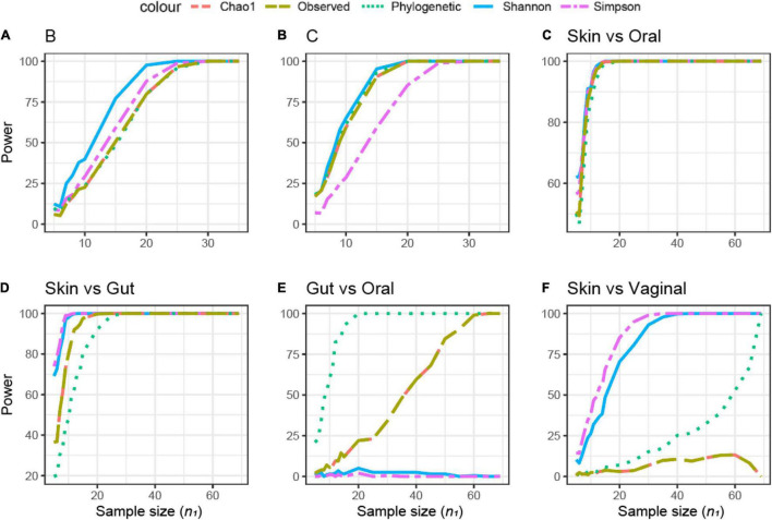
FIGURE 7 Empirical power of a two-sample Kruskal–Wallis test for the univariate comparison of two experimental microbiome datasets X1 and X2 from the Human Microbiome Projects (skin, gut, oral, and vaginal microbiome: dataset characteristics are given in Table 1). Differences between any two datasets X1 and X2 is assessed using different alpha diversity metrics [observed richness, phylogenetic diversity, Chao1, Shannon’s, and Simpson’s indices; see Equations (2)–(5), and (6) in section “Materials and Methods”]. The empirical power is calculated using Equation (11). Empirical power is calculated as a function of the sample size n1 of group 1 (with n2 = n1 and total sample size n = n1 + n2) using K = 1,000 replications (resampling)/tests for each sample size. (A–F) Different pairwise comparisons [A (poultry dataset B, feed A vs. B); B (poultry dataset C, feed A vs. B), skin microbiome vs. oral microbiome, skin vs. gut, gut vs. oral, and skin vs. vaginal].
FIGURE 7 Empirical power of a two-sample Kruskal–Wallis test for the univariate comparison of two experimental microbiome datasets X1 and X2 from the Human Microbiome Projects (skin, gut, oral, and vaginal microbiome: dataset characteristics are given in Table 1). Differences between any two datasets X1 and X2 is assessed using different alpha diversity metrics [observed richness, phylogenetic diversity, Chao1, Shannon’s, and Simpson’s indices; see Equations (2)–(5), and (6) in section “Materials and Methods”]. The empirical power is calculated using Equation (11). Empirical power is calculated as a function of the sample size n1 of group 1 (with n2 = n1 and total sample size n = n1 + n2) using K = 1,000 replications (resampling)/tests for each sample size. (A–F) Different pairwise comparisons [A (poultry dataset B, feed A vs. B); B (poultry dataset C, feed A vs. B), skin microbiome vs. oral microbiome, skin vs. gut, gut vs. oral, and skin vs. vaginal].CC BY · PubMed Central
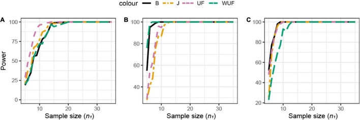
FIGURE 8 Empirical power of a two-sample Kruskal–Wallis test for the univariate comparison of two experimental microbiome datasets X1 and X2 from the three chicken datasets illustrated in Table 1. Differences between any two datasets X1 and X2 are assessed using different beta diversity metrics [Bray–Curtis dissimilarity (B), Jaccard (J), unweighted UniFrac (UF), and weighted UniFrac (WUF) distances; see Equations (7)–(9) and (6) in section “Materials and Methods”]. The empirical power is calculated using Equation (11) as a function of the sample size n1 of group 1 (with n2 = n1 and total sample size n = n1 + n2) using K = 100 replications. (A) Analysis of chicken dataset A. (B) Analysis of chicken dataset B. (C) Analysis of chicken dataset C.
FIGURE 8 Empirical power of a two-sample Kruskal–Wallis test for the univariate comparison of two experimental microbiome datasets X1 and X2 from the three chicken datasets illustrated in Table 1. Differences between any two datasets X1 and X2 are assessed using different beta diversity metrics [Bray–Curtis dissimilarity (B), Jaccard (J), unweighted UniFrac (UF), and weighted UniFrac (WUF) distances; see Equations (7)–(9) and (6) in section “Materials and Methods”]. The empirical power is calculated using Equation (11) as a function of the sample size n1 of group 1 (with n2 = n1 and total sample size n = n1 + n2) using K = 100 replications. (A) Analysis of chicken dataset A. (B) Analysis of chicken dataset B. (C) Analysis of chicken dataset C.CC BY · PubMed Central
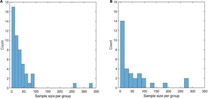
FIGURE 9 (A) Distribution of the sample size (per compared group) of the datasets that were analyzed, using the Chao1 diversity measure, in 28 of the 100 papers considered in the literature review. (A,B) Distribution of the sample size (per compared group) of the datasets that were analyzed, using permutational multivariate ANOVA (PERMANOVA), in 28 of the 100 papers considered in the literature review.
FIGURE 9 (A) Distribution of the sample size (per compared group) of the datasets that were analyzed, using the Chao1 diversity measure, in 28 of the 100 papers considered in the literature review. (A,B) Distribution of the sample size (per compared group) of the datasets that were analyzed, using permutational multivariate ANOVA (PERMANOVA), in 28 of the 100 papers considered in the literature review.CC BY · PubMed Central

Verification

Claims the paper makes

The claims and statistics of this paper haven’t been checked yet.

Run the check — free, no account needed. It reads the open-access text and checks the sources it cites.

A few free checks a day · papers already verified open instantly · results are public

Claims other papers make about this one

Each is checked against this paper’s own text: does it say what the citing paper says it does?

Self-check

Percentages, sums and reported differences re-computed from the paper’s own numbers.

The self-check needs the paper’s full text.

Citations

Cites

Show all 70 references

Research works printed but not linked: 6

  1. 1994, Publication Manual of the American Psychological Association: DAR ALMHRER ELADABE.
  2. Hoffman, 2015, Baic Biostatistics for Medical and Biomedical Practitioners.
  3. Kolassa, 2020, MultNonParam-Package R Documentation.
  4. Lahti, 2017, Tools for Microbiome Analysis in R. Microbiome Package Version 1.15.1.
  5. 2008, R: A Language and Environment for Statistical Computing.
  6. Shetty Sudarshan, 2020, Microbial Bioinformatics Introductory Course Material 2018 (Version v3.0).

Cited by

Sorted by citations

See all 361

Metadata

Authors
Kers, J. G., & Saccenti, E.
Affiliations
Wageningen University & Research (NL)
Corresponding author
Saccenti, Edoardo
Venue
Frontiers in Microbiology
Published
2022-03-03
Volume
12
Pages
796025-796025
ISSN
1664-302X (ISSN-L)
OpenAlex
W4214875183
Cited by
359
References
70
Citations by year
2026: 121 · 2025: 121 · 2024: 81 · 2023: 31 · 2022: 5
FWCI
19.51
Type
journal article
Language
en
Open access
Locations
  • Frontiers in Microbiology (publishedVersion, cc-by)
  • Research Square (acceptedVersion, cc-by)
  • PubMed Central (publishedVersion, cc-by)
  • PubMed (publishedVersion)
  • Socio-Environmental Systems Modeling (acceptedVersion, cc-by)
  • DOAJ (DOAJ: Directory of Open Access Journals) (submittedVersion, cc-by-sa)
  • Data Archiving and Networked Services (DANS) (submittedVersion, cc-by)
Funders
  • Nederlandse Organisatie voor Wetenschappelijk Onderzoek
  • European Commission
Topics
  • Life Sciences › Biochemistry, Genetics and Molecular Biology › Molecular Biology › Gut microbiota and health
  • Physical Sciences › Environmental Science › Ecology › Microbial Community Ecology and Physiology
  • Health Sciences › Dentistry › Periodontics › Oral microbiology and periodontitis research
Keywords
microbiome, sample size determination, statistical power, 16S rRNA amplicon sequencing, Bray-Curtis distance, p-hacking, publication bias, statistical reporting, pre-analysis plan

About these checks

Registry, retraction, Cites and statistics results are computed, not judged, with one exception: a printed reference that no index lists is read once by a model before it counts as a citation error. Claims are extracted by a model and kept only when their quote appears verbatim in the text; each cited source is then checked, with a model’s help, for whether it says what the claim relies on. Those verdicts can be wrong — read the claim’s quote and the cited source before relying on one.

Statistics and arithmetic are recomputed, not judged.

Confidence bands are shown only for fields calibrated on our annotated test set. None is calibrated yet, so no band is shown.

What counts as a claim ›How we measure confidence ›How we check this ›

Are you an author, or do you see a problem with this page? Request a review