

The DOI matches its Crossref record; 50 of the 50 references it cites were found in a registry or an index; none of the 30 sources its claims cite is checked for support yet.
Automated Conflation of Digital Elevation Model with Reference Hydrographic Lines
Open accessAbstract
Combining misaligned spatial data from different sources complicates spatial analysis and creation of maps. Conflation is a process that solves the misalignment problem through spatial adjustment or attribute transfer between similar features in two datasets. Even though a combination of digital elevation model (DEM) and vector hydrographic lines is a common practice in spatial analysis and mapping, no method for automated conflation between these spatial data types has been developed so far. The problem of DEM and hydrography misalignment arises not only in map compilation, but also during the production of generalized datasets. There is a lack of automated solutions which can ensure that the drainage network represented in the surface of generalized DEM is spatially adjusted with independently generalized vector hydrography. We propose a new method that performs the conflation of DEM with linear hydrographic data and is embeddable into DEM generalization process. Given a set of reference hydrographic lines, our method automatically recognizes the most similar paths on DEM surface called counterpart streams. The elevation data extracted from DEM is then rubbersheeted locally using the links between counterpart streams and reference lines, and the conflated DEM is reconstructed from the rubbersheeted elevation data. The algorithm developed for extraction of counterpart streams ensures that the resulting set of lines comprises the network similar to the network of ordered reference lines. We also show how our approach can be seamlessly integrated into a TIN-based structural DEM generalization process with spatial adjustment to pre-generalized hydrographic lines as additional requirement. The combination of the GEBCO_2019 DEM and the Natural Earth 10M vector dataset is used to illustrate the effectiveness of DEM conflation both in map compilation and map generalization workflows. Resulting maps are geographically correct and are aesthetically more pleasing in comparison to a straightforward combination of misaligned DEM and hydrographic lines without conflation.
Overview
CoChat Summary
TL;DR
The paper proposes an automated method to conflate digital elevation models with reference hydrographic lines by extracting counterpart streams on the DEM surface, rubbersheeting vectorized elevation data, and reconstructing the DEM, with integration into structural DEM generalization. Tests with GEBCO_2019 and Natural Earth 1:10M data show improved alignment and moderate displacement.
Key findings
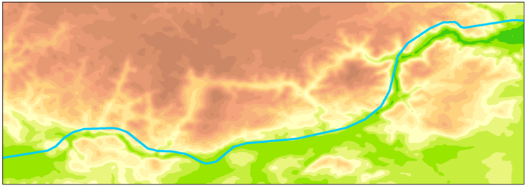
- The method aligns DEM with reference hydrographic lines without burning new terrain features; on a Central Europe test area (GEBCO_2019 DEM, 1358 × 1007 pixels, 28 Natural Earth 1:10M hydrographic features), all counterpart streams except one fell into the strong class limited by Fréchet distance, even though weak Directed Hausdorff constraints were used by default.
- Cohen’s kappa agreement between reference hydrographic lines and the DEM-derived drainage network increased on average from 0.56 (moderate) to 0.98 (almost perfect) after conflation.
- Total processing time for the non-generalized example was approximately 21.5 min; counterpart extraction took 17 min (79% of total), with flowline tracing taking 33 s and least-cost tracing taking 8 min 29 s in total.
- Displacement was moderate: mean horizontal displacement was 467 m and median 302 m; 66% of elevation points moved no farther than the DEM pixel size, and 95% moved no farther than 1480 m. Vertical displacement had mean 0.07 m, median 0.03 m, and 95% of absolute vertical displacements were no greater than 27.42 m.
Methods
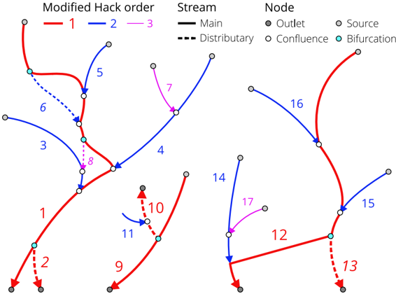
- Design: a seven-stage workflow—order reference hydrographic lines using modified Hack ordering, trace counterpart streams via flowline and least-cost approaches, generate rubbersheet links, extract elevation data as vector features, rubbersheet the elevation data, build a TIN, reconstruct the conflated DEM, and optionally carve/widen along reference lines.
- Data and sample: GEBCO_2019 raster DEM at 15 arc-seconds (approximately 500 m along the equator) and Natural Earth 1:10,000,000 hydrography (version 4.1.0), clipped to Central Europe mainly in the Danube basin; parameters used were catch radius r = 6000, minimum flow accumulation a = 10, and offstream penalty weight w = 30.
- Main analysis: visual map comparison and Cohen’s kappa agreement between reference lines and drainage networks extracted from source versus conflated DEMs, plus displacement statistics for rubbersheeted elevation points.
Limitations
- Stated in the paper: least-cost counterparts can only be constrained by the weak Directed Hausdorff distance in the current map-algebra implementation, and unreliable counterparts can occur in densely packed meanders with large catch radius (Figure 19); no tiling solution exists yet for large datasets; accuracy change from displacement is unclear; analysis of geomorphometric and hydrological derivatives is out of scope; additional experiments are needed when hydrography is more detailed than the DEM.
- Evident from the text: the method is demonstrated on one coarse-resolution DEM and one generalized hydrography dataset in Central Europe, with parameters selected experimentally; processing time is dominated by the Python/arcpy implementation, and the paper does not report independent validation of hydrological or geomorphometric accuracy beyond displacement statistics and kappa agreement.
Model-written summary. Check it against the paper before relying on it.
Integrity signals
Registry
Cites
Statistics
Figures






Verification
Claims the paper makes
0 Valid · 5 Not valid · 23 Not checked · 108 Own results and interpretations
A result the paper states — it cites no source for it, so there is none to check. The quote shows it is in the paper.
In the paper
“At the same time, duration of least-cost counterpart tracing showed no dependency on catch radius.”
§ Automated Conflation of Digital Elevation Model with Reference Hydrographic Lines > Processing Time
plain- Asserted: passes — The authors put it forward as true.
- Checkable: passes — It can be checked against evidence.
- Load-bearing: unclear — It is unclear whether the paper’s conclusions depend on it.
- Based: passes — The paper gives a reason why it holds.
A result the paper reports from its own data — it cites no other source for it, so there is none to check. The quote shows it is in the paper.
In the paper
“Duration of tracing the flowline counterpart streams showed power law dependency on the value of catch radius r.”
§ Automated Conflation of Digital Elevation Model with Reference Hydrographic Lines > Processing Time
plainstates an associationSingle case- Asserted: passes — The authors put it forward as true.
- Checkable: passes — It can be checked against evidence.
- Load-bearing: unclear — It is unclear whether the paper’s conclusions depend on it.
- Based: passes — The paper gives a reason why it holds.
A result the paper reports from its own data — it cites no other source for it, so there is none to check. The quote shows it is in the paper.
In the paper
“Resulting values show that our method systematically improves the alignment between the reference hydrographic lines and the drainage network implicitly represented in DEM surface.”
§ Automated Conflation of Digital Elevation Model with Reference Hydrographic Lines > Results
plainstates a cause- Asserted: passes — The authors put it forward as true.
- Checkable: passes — It can be checked against evidence.
- Load-bearing: passes — The paper’s conclusions depend on it.
- Based: passes — The paper gives a reason why it holds.
- Rests on an assumption not shown here.
A result the paper reports from its own data — it cites no other source for it, so there is none to check. The quote shows it is in the paper.
In the paper
“The average value of index of agreement increased from 0.56 (moderate) to 0.98 (almost perfect) as a result of conflation.”
§ Automated Conflation of Digital Elevation Model with Reference Hydrographic Lines > Results
plainstates a cause- Asserted: passes — The authors put it forward as true.
- Checkable: passes — It can be checked against evidence.
- Load-bearing: passes — The paper’s conclusions depend on it.
- Based: passes — The paper gives a reason why it holds.
- Rests on an assumption not shown here.
A result the paper reports from its own data — it cites no other source for it, so there is none to check. The quote shows it is in the paper.
In the paper
“Our method effectively aligns DEM with reference hydrographic lines, which is demonstrated on multiple cartographic examples and substantiated by significant improvement of agreement statistics between the reference hydrographic lines and a drainage network on DEM surface.”
§ Automated Conflation of Digital Elevation Model with Reference Hydrographic Lines > A combination of flowline and least-cost approaches allows extraction of counterpart streams in a
boostedstates a cause- Asserted: passes — The authors put it forward as true.
- Checkable: passes — It can be checked against evidence.
- Load-bearing: passes — The paper’s conclusions depend on it.
- Based: passes — The paper gives a reason why it holds.
- Rests on an assumption not shown here.
39 more claims
Create a free account to see all 136 claims and to verify the 30 references still open.
- It may state two separate claims as one. 42
- Probably not a substantial claim. 63
- The quote only partly states this claim. 1
Self-check
Percentages, sums and reported differences re-computed from the paper’s own numbers.
Each contradiction between two passages listed here was confirmed by an independent check.
Rated minor: it would not touch a result — a value no result rests on, a p-value that stays on the same side of the significance level, or a conflict that is clerical, resolved elsewhere in the paper, or outside its own findings.
In the paper
§ Automated Conflation of Digital Elevation Model with Reference Hydrographic Lines > Results
“distributary least-cost streams (ID = 9, 34)”
§ Automated Conflation of Digital Elevation Model with Reference Hydrographic Lines > A combination of flowline and least-cost approaches allows extraction of counterpart streams in a
“| 34 | 12 | -1 | 3 | 3 Main | Least-cost | 4417 | 4417 | 4417 Strong |”
Citations
Cites
A Coefficient of Agreement for Nominal Scales
Cohen, J. (1960) · Educational and Psychological Measurement · doi:10.1177/001316446002000104 · Cited by 42,398
The extraction of drainage networks from digital elevation data
O'Callaghan, J. F., & Mark, D. M. (1984) · Computer Vision, Graphics, and Image Processing · doi:10.1016/s0734-189x(84)80011-0 · Cited by 2,752
A modified Hausdorff distance for object matching
Dubuisson, M.-P., & Jain, A. K. (2002) · Proceedings of 12th International Conference on Pattern Recognition · doi:10.1109/icpr.1994.576361 · Cited by 1,464
A new procedure for gridding elevation and stream line data with automatic removal of spurious pits
Hutchinson, M. F. (1989) · Journal of Hydrology · doi:10.1016/0022-1694(89)90073-5 · Cited by 1,254
Global multi-resolution terrain elevation data 2010 (GMTED2010)
Danielson, J. J., & Gesch, D. B. (2011) · Open-File Report · doi:10.3133/ofr20111073 · Cited by 1,181
COMPUTING THE FRÉCHET DISTANCE BETWEEN TWO POLYGONAL CURVES
ALT, H., & GODAU, M. (1995) · International Journal of Computational Geometry & Applications · doi:10.1142/s0218195995000064 · Cited by 1,039
Sur quelques points du calcul fonctionnel
Fréchet, M. M. (1906) · Rendiconti del Circolo Matematico di Palermo · doi:10.1007/bf03018603 · Cited by 1,023
Map-matching for low-sampling-rate GPS trajectories
Lou, Y., Zhang, C., Zheng, Y., Xie, X., Wang, W., & Huang, Y. (2009) · Proceedings of the 17th ACM SIGSPATIAL International Conference on Advances in Geographic Information Systems · doi:10.1145/1653771.1653820 · Cited by 797
Assuring the quality of volunteered geographic information
Goodchild, M. F., & Li, L. (2012) · Spatial Statistics · doi:10.1016/j.spasta.2012.03.002 · Cited by 771
Wang, L., & Liu, H. (2006) · International Journal of Geographical Information Science · doi:10.1080/13658810500433453 · Cited by 506
Conflation Automated map compilation
Saalfeld, A. (1988) · International Journal of Geographical Information Systems · doi:10.1080/02693798808927897 · Cited by 298
Matching spatial data sets: a statistical approach
WALTER, V., & FRITSCH, D. (1999) · International Journal of Geographical Information Science · doi:10.1080/136588199241157 · Cited by 287
Lindsay, J. B. (2015) · Hydrological Processes · doi:10.1002/hyp.10648 · Cited by 193
A Rule-based Approach for the Conflation of Attributed Vector Data
Cobb, M. A., Chung, M. J., Foley, H., Petry, F. E., Shaw, K., & Miller, H. V. (1998) · GeoInformatica · doi:10.1023/a:1009788905049 · Cited by 180
Least-cost Path in GIS Using an Accumulated Cost Surface and Slopelines
DOUGLAS, D. H. (1994) · Cartographica · doi:10.3138/d327-0323-2jut-016m · Cited by 177
Matching Networks with Different Levels of Detail
Mustière, S., & Devogèle, T. (2007) · GeoInformatica · doi:10.1007/s10707-007-0040-1 · Cited by 166
Carving and adaptive drainage enforcement of grid digital elevation models
Soille, P., Vogt, J., & Colombo, R. (2003) · Water Resources Research · doi:10.1029/2002wr001879 · Cited by 132
Geostatistics for conflation and accuracy assessment of digital elevation models
Kyriakidis, P. C., Shortridge, A. M., & Goodchild, M. F. (1999) · International Journal of Geographical Information Systems · doi:10.1080/136588199241067 · Cited by 131
Generalization of DEM for terrain analysis using a compound method
Zhou, Q., & Chen, Y. (2010) · ISPRS Journal of Photogrammetry and Remote Sensing · doi:10.1016/j.isprsjprs.2010.08.005 · Cited by 123
An optimisation model for linear feature matching in geographical data conflation
Li, L., & Goodchild, M. F. (2011) · International Journal of Image and Data Fusion · doi:10.1080/19479832.2011.577458 · Cited by 115
The Practice of DEM Stream Burning Revisited
Lindsay, J. B. (2016) · Earth Surface Processes and Landforms · doi:10.1002/esp.3888 · Cited by 106
Burghardt, D., Duchêne, C., & Mackaness, W. (2014) · Lecture notes in geoinformation and cartography · doi:10.1007/978-3-319-00203-3 · Cited by 98
Automatically Conflating Road Vector Data with Orthoimagery
Chen, C.-C., Knoblock, C. A., & Shahabi, C. (2006) · GeoInformatica · doi:10.1007/s10707-006-0344-6 · Cited by 91
A DEM generalization by minor valley branch detection and grid filling
Ai, T., & Li, J. (2009) · ISPRS Journal of Photogrammetry and Remote Sensing · doi:10.1016/j.isprsjprs.2009.11.001 · Cited by 77
Piecewise Linear Rubber-Sheet Map Transformation
White, M. S., & Griffin, P. (1985) · The American Cartographer · doi:10.1559/152304085783915135 · Cited by 64
Comparison of drainage-constrained methods for DEM generalization
Chen, Y., Wilson, J. P., Zhu, Q., & Zhou, Q. (2012) · Computers & Geosciences · doi:10.1016/j.cageo.2012.05.002 · Cited by 60
Spatial data integrity constraints in object oriented geographic data modeling
Borges, K. A. V., Laender, A. H. F., & Davis, C. A., Jr. (1999) · ACM SIGSPATIAL International Conference on Advances in Geographic Information Systems (SIGSPATIAL GIS) · doi:10.1145/320134.320136 · Cited by 59
Qualitative matching of spatial information
Wallgrün, J. O., Wolter, D., & Richter, K. (2010) · ACM SIGSPATIAL International Conference on Advances in Geographic Information Systems (SIGSPATIAL GIS) · doi:10.1145/1869790.1869833 · Cited by 58
Wu, T., Li, J., Li, T., Sivakumar, B., Zhang, G., & Wang, G. (2019) · Geomorphology · doi:10.1016/j.geomorph.2019.04.022 · Cited by 51
Jordán, G. (2007) · Computers & Geosciences · doi:10.1016/j.cageo.2006.08.010 · Cited by 50
Improving Hydrological Information Acquisition from DEM Processing in Floodplains
Getirana, A. C. V., Bonnet, M., Rotunno Filho, O. C., & Mansur, W. J. (2009) · Hydrological Processes · doi:10.1002/hyp.7167 · Cited by 44
Generalisation in Practice Within National Mapping Agencies
Duchêne, C., Baella, B., Brewer, C. A., Burghardt, D., Buttenfield, B. P., Gaffuri, J., Käuferle, D., Lecordix, F., Maugeais, E., Nijhuis, R., et al. (2014) · Lecture notes in geoinformation and cartography · doi:10.1007/978-3-319-00203-3_11 · Cited by 43
Conflation of OpenStreetMap and Mobile Sports Tracking Data for Automatic Bicycle Routing
Bergman, C., & Oksanen, J. (2016) · Transactions in GIS · doi:10.1111/tgis.12192 · Cited by 37
Tomlin, C. (2012) · Cited by 36
Automatic generation of hypsometric layers for small-scale maps
Leonowicz, A. M., Jenny, B., & Hurni, L. (2009) · Computers & Geosciences · doi:10.1016/j.cageo.2008.12.012 · Cited by 33
Optimal spatial data matching for conflation: A network flow‐based approach
Lei, T., & Lei, Z. (2019) · Transactions in GIS · doi:10.1111/tgis.12561 · Cited by 28
Map-Matching Using Shortest Paths
Chambers, E. W., Fasy, B. T., Wang, Y., & Wenk, C. (2020) · ACM Transactions on Spatial Algorithms and Systems · doi:10.1145/3368617 · Cited by 22
Stanislawski, L. V., Survila, K., Wendel, J., Liu, Y., & Buttenfield, B. P. (2017) · Cartography and Geographic Information Science · doi:10.1080/15230406.2017.1337524 · Cited by 19
A rapid approach for automated comparison of independently derived stream networks
Stanislawski, L. V., Buttenfield, B. P., & Doumbouya, A. (2015) · Cartography and Geographic Information Science · doi:10.1080/15230406.2015.1060869 · Cited by 18
Advances in Cartography and GIScience. Volume 1: Selection from ICC 2011, Paris
Savino, S., M, R., Fabio, C., Langiu, G., & Raineri, M. (2011) · Lecture notes in geoinformation and cartography · doi:10.1007/978-3-642-19143-5 · Cited by 17
Multi-resolution representation of digital terrain models with terrain features preservation
Li, Q., Wang, Z., & Yang, B. (2008) · Science China Technological Sciences · doi:10.1007/s11431-008-5015-4 · Cited by 16
A New DEM Generalization Method Based on Watershed and Tree Structure
Chen, Y.-G., Ma, T., Chen, X., Chen, Z., Yang, C.-J., Lin, C., & Shan, L. (2016) · PLoS ONE · doi:10.1371/journal.pone.0159798 · Cited by 14
Stream Network Conflation with Topographic DEMs
Yadav, B., & Hatfield, K. (2018) · Environmental Modelling & Software · doi:10.1016/j.envsoft.2018.01.009 · Cited by 14
A general framework for conflation
Adams, B., Li, L., Raubal, M., & Goodchild, M. F. (2010) · UC Research Repository (University of Canterbury) · Cited by 12
Minimizing Walking Length in Map Matching
Gheibi, A., Maheshwari, A., & Sack, J.-R. (2016) · Lecture notes in computer science · doi:10.1007/978-3-319-28678-5_8 · Cited by 10
Arundel, S. T., Thiem, P. T., & Constance, E. W. (2018) · Cartography and Geographic Information Science · doi:10.1080/15230406.2016.1230027 · Cited by 8
DEM generalization based on analysis of geometry and landscape context
Fan, Q., Li, Y., & Hu, P. (2007) · Proceedings of SPIE, the International Society for Optical Engineering/Proceedings of SPIE · doi:10.1117/12.750728 · Cited by 5
Conflation in Geoprocessing Framework – Case Studies Recent development and looking ahead
Lee, D., Yang, W., & Ahmed, N. (2014) · doi:10.13140/2.1.4454.5924 · Cited by 3
Samsonov, T. (2020) · Zenodo (CERN European Organization for Nuclear Research) · doi:10.5281/zenodo.3813731 · Cited by 1
Self-citation(1988) · Photogrammetric Engineering & Remote Sensing
Research works printed but not linked: 8
- Stanislawski, L.V., Nelson, C., and Hamann, M. (2002, January 8–12). Automated Conflation of Reach Data for the National Hydrography Dataset. Proceedings of the 22nd Annual Esri International User Conference, San Diego, CA, USA.
- Revell, P., Regnauld, N., and Bulbrooke, G. (2011, January 3–8). OS VectorMapTM District: Automated Generalisation, Text Placement and Conflation in Support of Making Pubic Data Public. Proceedings of the 25th International Cartographic Conference, Paris, France.
- (2020, May 10). GEBCO 2019 Grid. Available online: https://www.bodc.ac.uk/data/published_data_library/catalogue/10.5285/836f016a-33be-6ddc-e053-6c86abc0788e/. · doi:10.5285/836f016a-33be-6ddc-e053-6c86abc0788e/
- Saunders, W. (2020, May 10). Preparation of DEMs for Use in Environmental Modeling Analysis. Available online: https://proceedings.esri.com/library/userconf/proc99/proceed/papers/pap802/p802.htm.
- Burghardt, D., Duchêne, C., and Mackaness, W. (2014). Terrain Generalisation. Abstracting Geographic Information in a Data Rich World, Springer International Publishing. · DOI
- Weibel, R. (April, January 29). An Adaptive Methodology for Automated Relief Generalization. Proceedings of the AutoCarto 8, Baltimore, MD, USA.
- Gaffuri, J. (2007, January 10–12). Field Deformation in an Agent-Based Generalisation Model: The GAEL Model. Proceedings of the 5th Geographic Information Days, Münster, Germany.
- Tomlin, D. (2012). GIS and Cartographic Model, ESRI Press. [2nd ed.].
Cited by
Geomorphometry and terrain analysis: data, methods, platforms and applications
Xiong, L., Li, S., Tang, G., & Strobl, J. (2022) · Earth-Science Reviews · doi:10.1016/j.earscirev.2022.104191 · Cited by 160
Huang, F., Yang, J., Zhang, B., Li, Y., Huang, J., & Chen, N. (2020) · ISPRS International Journal of Geo-Information · doi:10.3390/ijgi9090539 · Cited by 25
Terrain generalization with line integral convolution
Jenny, B. (2020) · Cartography and Geographic Information Science · doi:10.1080/15230406.2020.1833762 · Cited by 23
Song, S., & Qin, R. (2023) · IEEE Geoscience and Remote Sensing Letters · doi:10.1109/lgrs.2023.3298321 · Cited by 6
The experience of creating a database in a GIS environment
Ivlieva, N., Федорович, М. В., Boriskin, A. S., & Erofeeva, I. V. (2021) · Geodesy and Cartography · doi:10.22389/0016-7126-2020-966-12-43-49 · Cited by 3
Metadata
- Authors
- Samsonov, T. E.
- Affiliations
- Lomonosov Moscow State University (RU)
- Corresponding author
- Samsonov, Timofey E.
- ORCID
- Samsonov, Timofey E.
- Venue
- ISPRS International Journal of Geo-Information
- Publisher
- MDPI AG
- Published
- 2020-05-20
- Volume
- 9
- Issue
- 5
- Pages
- 334
- ISSN
- 2220-9964 (ISSN-L)
- OpenAlex
- W3027522656
- Cited by
- 15
- References
- 50
- Citations by year
- 2026: 1 · 2025: 2 · 2024: 3 · 2023: 1 · 2022: 2 · 2021: 4 · 2020: 2
- FWCI
- 4.14
- Type
- journal article
- Language
- en
- Open access
- gold
- dx.doi.org
- Licence
- Locations
- ISPRS International Journal of Geo-Information (publishedVersion, cc-by)
- DOAJ (DOAJ: Directory of Open Access Journals) (submittedVersion, cc-by-sa)
- Funders
- Russian Science Foundation (19-77-00071)
- Topics
- Social Sciences › Geography, Planning and Development › Geographic Information Systems Studies
- Social Sciences › Geography, Planning and Development › Historical Geography and Cartography
- Physical Sciences › Computer Science › Computer Vision and Pattern Recognition › Satellite Image Processing and Photogrammetry
- Keywords
- digital elevation model, rubber sheeting, spatial adjustment, drainage network, map compilation
About these checks
Registry, retraction, Cites and statistics results are computed, not judged, with one exception: a printed reference that no index lists is read once by a model before it counts as a citation error. Claims are extracted by a model and kept only when their quote appears verbatim in the text; each cited source is then checked, with a model’s help, for whether it says what the claim relies on. Those verdicts can be wrong — read the claim’s quote and the cited source before relying on one.
A language model drew the claims from the paper on 2026-11-19, under version 3 of the claim definition (model deepseek-v4.1-flash, prompt extract-v3).
A second model labelled each claim on 2026-11-19 (model jev-1.13-20260917, definition revision gold-guideline-v0.2).
Statistics and arithmetic are recomputed, not judged.
Confidence bands are shown only for fields calibrated on our annotated test set. None is calibrated yet, so no band is shown.
What counts as a claim ›How we measure confidence ›How we check this ›
Are you an author, or do you see a problem with this page? Request a review
Data sources
Bibliographic data: Semantic Scholar, OpenAlex, Crossref.
Contains information from the Semantic Scholar Academic Graph Datasets, made available under the ODC Attribution License (ODC-BY 1.0).
Semantic Scholar’s data is described in: Kinney, R., et al. (2023). The Semantic Scholar Open Data Platform. arXiv:2301.10140.
