

The DOI matches its Crossref record.
Sky-View Factor as a Relief Visualization Technique
Abstract
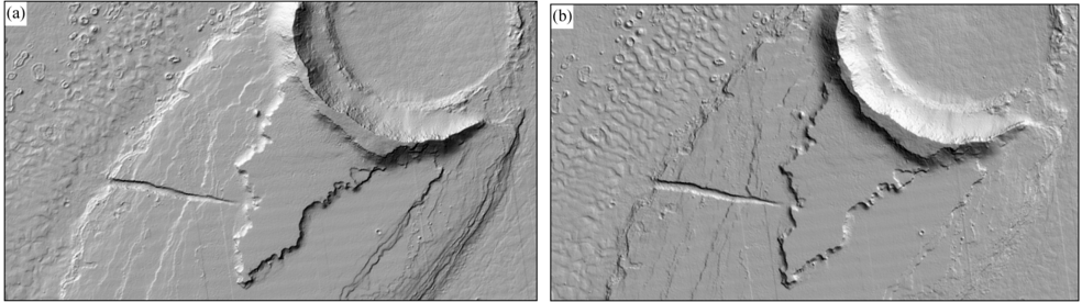
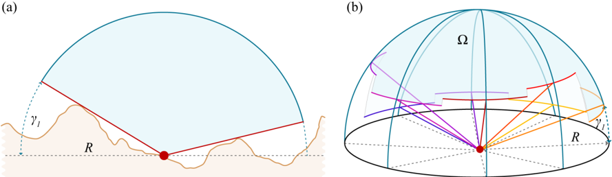
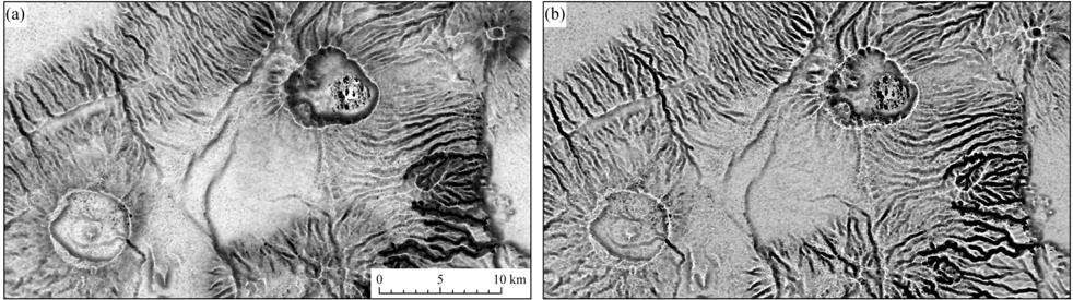
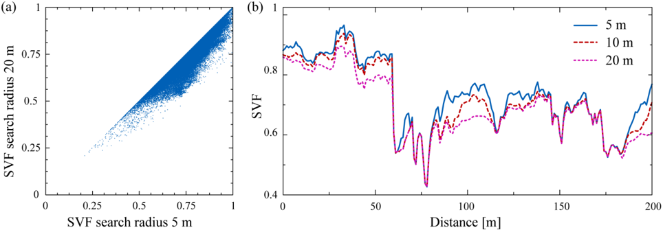
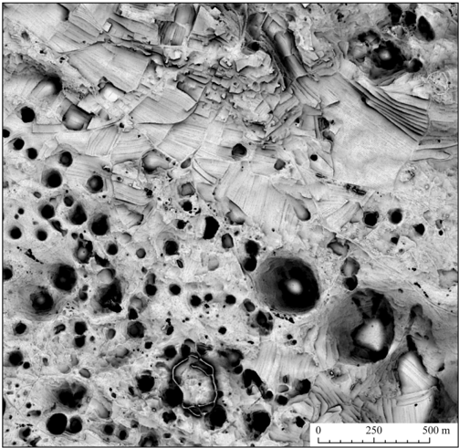
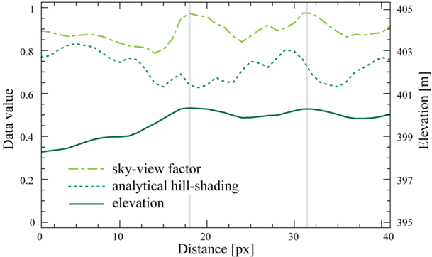
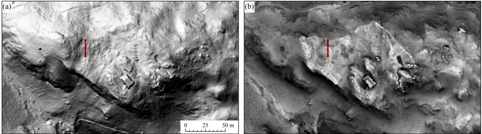
Remote sensing has become the most important data source for the digital elevation model (DEM) generation. DEM analyses can be applied in various fields and many of them require appropriate DEM visualization support. Analytical hill-shading is the most frequently used relief visualization technique. Although widely accepted, this method has two major drawbacks: identifying details in deep shades and inability to properly represent linear features lying parallel to the light beam. Several authors have tried to overcome these limitations by changing the position of the light source or by filtering. This paper proposes a new relief visualization technique based on diffuse, rather than direct, illumination. It utilizes the sky-view factor—a parameter corresponding to the portion of visible sky limited by relief. Sky-view factor can be used as a general relief visualization technique to show relief characteristics. In particular, we show that this visualization is a very useful tool in archaeology as it improves the recognition of small scale features from high resolution DEMs.
Overview
The claims and statistics of this paper haven’t been checked yet.
Run the check — free, no account needed. It reads the open-access text and checks the sources it cites.
Integrity signals
Registry
Cites
Statistics
Figures
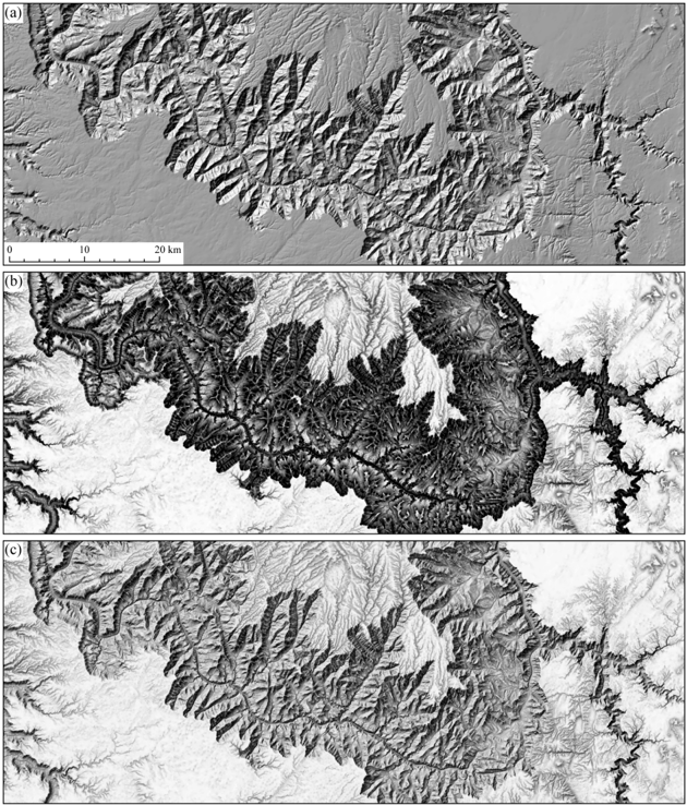
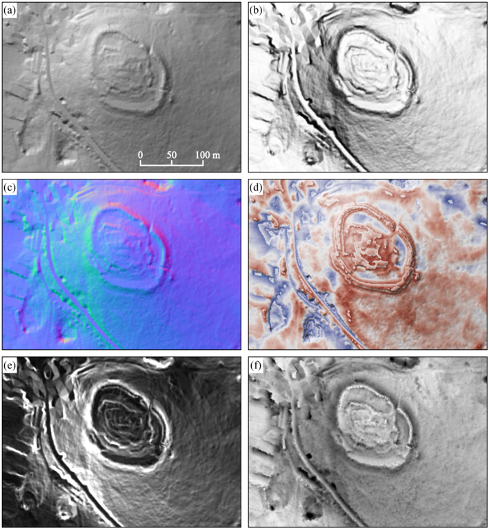
Verification
Claims the paper makes
The claims and statistics of this paper haven’t been checked yet.
Run the check — free, no account needed. It reads the open-access text and checks the sources it cites.
Claims other papers make about this one
Each is checked against this paper’s own text: does it say what the citing paper says it does?
In the citing paper
“Due to these limitations, the Rhineland Commission for Archaeological Monuments and Sites in Bonn mainly works with RVT [Kokalj et al. 2011;Zakšek et al. 2011].”
From Reconstructing Pre-Industrial Long Distance Roads in a Hilly Region in Germany, Based on Historical and Archaeological Data (2017) · cites this paper as Zakšek et al. 2011
Self-check
Percentages, sums and reported differences re-computed from the paper’s own numbers.
The self-check needs the paper’s full text.
Citations
Cites
No references could be resolved yet.
Research works printed but not linked: 44
- Kirk, 2008, Ultrahigh resolution topographic mapping of Mars with MRO HiRISE stereo images: Meter-scale slopes of candidate Phoenix landing sites, J. Geophys. Res., 113, E00A24, 10.1029/2007JE003000 · DOI
- Burrough, P.A., and McDonnell, R.A. (1998). Principles of Geographical Information Systems, Oxford University Press. [2nd ed.].
- Podobnikar, 2005, Solar radiation modelling, Comput. Geosci., 31, 233, 10.1016/j.cageo.2004.09.018 · DOI
- Jain, 2005, DEM-based modelling of surface runoff using diffusion wave equation, J. Hydrol., 302, 107, 10.1016/j.jhydrol.2004.06.042 · DOI
- Chaplot, 2005, Impact of DEM mesh size and soil map scale on SWAT runoff, sediment, and NO3-N loads predictions, J. Hydrol., 312, 207, 10.1016/j.jhydrol.2005.02.017 · DOI
- Kokalj, 2011, Application of sky-view factor for the visualization of historic landscape features in lidar-derived relief models, Antiquity, 85, 263, 10.1017/S0003598X00067594 · DOI
- Horn, 1981, Hill shading and the reflectance map, Proc. IEEE, 69, 14, 10.1109/PROC.1981.11918 · DOI
- Jenny, 2001, An interactive approach to analytical relief shading, Cartographica, 38, 67, 10.3138/F722-0825-3142-HW05 · DOI
- Patterson, 1997, A desktop approach to shaded relief production, Cartogr. Perspect., 28, 38, 10.14714/CP28.694 · DOI
- Price, 2001, Relief presentation: Manual airbrushing combined with computer technology, Cartogr. J., 38, 107, 10.1179/caj.2001.38.1.107 · DOI
- Horn, 1981, Hill shading and the reflectance map, Proc. IEEE, 69, 14, 10.1109/PROC.1981.11918 · DOI
- Phong, 1975, Illumination for computer generated pictures, Commun. ACM, 18, 311, 10.1145/360825.360839 · DOI
- Blinn, 1977, Models of light reflection for computer synthesized pictures, SIGGRAPH Comput. Graph., 11, 192, 10.1145/965141.563893 · DOI
- Batson, 1975, Computer generated shaded relief images, J. Res. US Geol. Surv., 3, 401
- Kuiper, G.P., and Middlehurst, B.M. (1961). Planets and Satellites, The University of Chicago Press.
- 1965, Analytische Schattierung, Ein kartographischer Entwurf. Kartographische Nachrichten, 15, 141
- Devereux, 2008, Visualisation of LiDAR terrain models for archaeological feature detection, Antiquity, 82, 470, 10.1017/S0003598X00096952 · DOI
- Brassel, 1974, A model for automatic hill-shading, Cartogr. Geogr. Inf. Sci., 1, 15
- Imhof, E. (1982). Cartographic Relief Presentation, Walter de Gruyter. · DOI
- Hobbs, 1995a, The rendering of relief images from digital contour data, Cartogr. J., 32, 111, 10.1179/caj.1995.32.2.111 · DOI
- Hobbs, 1999b, An investigation of RGB multi-band shading for relief visualisation, Int. J. Appl. Earth Obs. Geoinf., 1, 181
- Zhukov, S., Iones, A., and Korin, G. (July, January 29). An Ambient Light Illumination Model. Proceedings of Eurographics Rendering Workshop on Rendering Techniques, Vienna, Austria.
- Sbert, 2009, From obscurances to ambient occlusion: A survey, Visual Comput., 25, 181, 10.1007/s00371-008-0213-4 · DOI
- Sbert, 2008, Viewpoint-based ambient occlusion, IEEE Comput. Graph. Applications, 28, 44, 10.1109/MCG.2008.41 · DOI
- Ruiz, 2010, Volumetric ambient occlusion for volumetric models, Visual Comput., 26, 687, 10.1007/s00371-010-0497-z · DOI
- Yokoyama, 2002, Visualizing topography by openness: A new application of image processing to digital elevation models, Photogramm. Eng. Remote Sensing, 68, 251
- Kennelly, 2006, A uniform sky illumination model to enhance shading of terrain and urban areas, Cartogr. Geogr. Inform. Sci., 33, 21, 10.1559/152304006777323118 · DOI
- Steyn, 1980, The calculation of view factors from fisheye-lens photographs, Atmos. Ocean, 18, 254, 10.1080/07055900.1980.9649091 · DOI
- Goldberg, 2005, GIS-based regionalisation of radiation, temperature and coupling measures in complex terrain for low mountain ranges, Meteorol. Appl., 12, 33, 10.1017/S1350482705001489 · DOI
- Richards, 2006, Sky view and weather controls on nocturnal surface moisture deposition on grass at urban sites, Phys. Geogr., 27, 70, 10.2747/0272-3646.27.1.70 · DOI
- Oke, T.R. (1988). Boundary Layer Climates, Routledge. [2nd ed.].
- Marks, 1979, A clear-sky longwave radiation model for remote alpine areas, Arch. Met. Geoph. Biokl. Serie B, 27, 159, 10.1007/BF02243741 · DOI
- Eliasson, 1996, Urban nocturnal temperatures, street geometry and land use, Atmos. Environ., 30, 379, 10.1016/1352-2310(95)00033-X · DOI
- Bourbia, 2004, Building cluster and shading in urban canyon for hot dry climate: Part 1: Air and surface temperature measurements, Renewable Energy, 29, 249, 10.1016/S0960-1481(03)00170-8 · DOI
- Blennow, 1998, Modelling minimum air temperature in partially and clear felled forests, Agr. Forest Meteorol., 91, 223, 10.1016/S0168-1923(98)00069-0 · DOI
- Robinson, 2006, Urban morphology and indicators of radiation availability, Solar Energy, 80, 1643, 10.1016/j.solener.2006.01.007 · DOI
- Yard, 2005, Influence of topographic complexity on solar insolation estimates for the Colorado River, Grand Canyon, AZ, Ecol. Model., 183, 157, 10.1016/j.ecolmodel.2004.07.027 · DOI
- Dozier, 1981, A faster solution to the horizon problem, Comput. Geosci., 7, 145, 10.1016/0098-3004(81)90026-1 · DOI
- Kennelly, 2008, Terrain maps displaying hill-shading with curvature, Geomorphology, 102, 567, 10.1016/j.geomorph.2008.05.046 · DOI
- Challis, K., Forlin, P., and Kincey, M. (2011). A generic toolkit for the visualisation of archaeological features on airborne lidar elevation data. Archaeol. Prospect., in print. · DOI
- Wood, J. (1996). The Geomorphological Characterization of Digital Elevation Models. [Ph.D. Thesis, University of Leicester]. Available online: http://www.soi.city.ac.uk/~jwo/phd.
- Hesse, 2010, LiDAR-derived Local Relief Models—A new tool for archaeological prospection, Archaeol. Prospect., 17, 67, 10.1002/arp.374 · DOI
- Corripio, 2003, Vectorial algebra algorithms for calculating terrain parameters from DEMs and solar radiation modelling in mountainous terrain, Int. J. Geogr. Inf. Sci., 17, 1, 10.1080/713811744 · DOI
- Revfeim, 1978, A simple procedure for estimating global daily radiation on any surface, J. Appl. Meteorol., 17, 1126, 10.1175/1520-0450(1978)017<1126:ASPFEG>2.0.CO;2 · DOI
Cited by
Sorted by citations
Herzog, I. (2017) · Studies in Digital Heritage · doi:10.14434/sdh.v1i2.23283 · Cited by 21
Metadata
- Authors
- Zakšek, K., Oštir, K., & Kokalj, Ž.
- Affiliations
- Institute of Geophysics, University of Hamburg, Bundesstr. 55, D-20146 Hamburg, Germany
- Centre of Excellence Space-SI, Aškerčeva cesta 12, SI-1000 Ljubljana, Slovenia
- Venue
- Remote Sensing
- Publisher
- MDPI AG
- Published
- 2011-02-23
- Volume
- 3
- Issue
- 2
- Pages
- 398-415
- ISSN
- 2072-4292
- Cited by
- 562
- References
- 0
- Language
- en
About these checks
Registry, retraction, Cites and statistics results are computed, not judged, with one exception: a printed reference that no index lists is read once by a model before it counts as a citation error. Claims are extracted by a model and kept only when their quote appears verbatim in the text; each cited source is then checked, with a model’s help, for whether it says what the claim relies on. Those verdicts can be wrong — read the claim’s quote and the cited source before relying on one.
Statistics and arithmetic are recomputed, not judged.
Confidence bands are shown only for fields calibrated on our annotated test set. None is calibrated yet, so no band is shown.
What counts as a claim ›How we measure confidence ›How we check this ›
Are you an author, or do you see a problem with this page? Request a review
