

The DOI matches its DataCite record.
MultiScale MeshGraphNets
Abstract
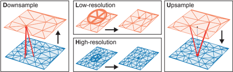
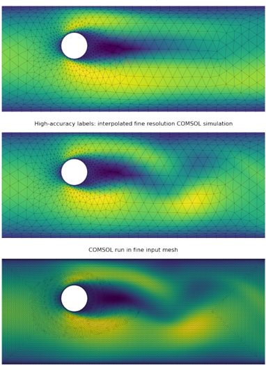
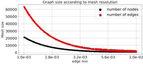
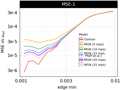
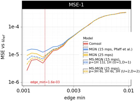
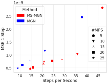
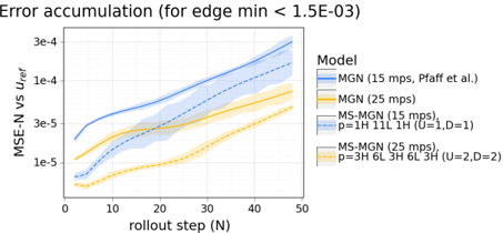
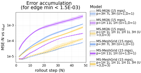
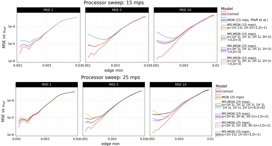
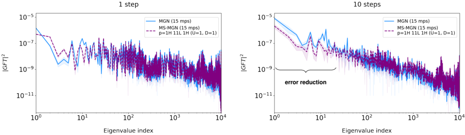
In recent years, there has been a growing interest in using machine learning to overcome the high cost of numerical simulation, with some learned models achieving impressive speed-ups over classical solvers whilst maintaining accuracy. However, these methods are usually tested at low-resolution settings, and it remains to be seen whether they can scale to the costly high-resolution simulations that we ultimately want to tackle. In this work, we propose two complementary approaches to improve the framework from MeshGraphNets, which demonstrated accurate predictions in a broad range of physical systems. MeshGraphNets relies on a message passing graph neural network to propagate information, and this structure becomes a limiting factor for high-resolution simulations, as equally distant points in space become further apart in graph space. First, we demonstrate that it is possible to learn accurate surrogate dynamics of a high-resolution system on a much coarser mesh, both removing the message passing bottleneck and improving performance; and second, we introduce a hierarchical approach (MultiScale MeshGraphNets) which passes messages on two different resolutions (fine and coarse), significantly improving the accuracy of MeshGraphNets while requiring less computational resources.
Overview
The claims and statistics of this paper haven’t been checked yet.
Run the check — free, no account needed. It reads the open-access text and checks the sources it cites.
Integrity signals
Registry
Cites
Statistics
Figures
Verification
Claims the paper makes
The claims and statistics of this paper haven’t been checked yet.
Run the check — free, no account needed. It reads the open-access text and checks the sources it cites.
Claims other papers make about this one
Each is checked against this paper’s own text: does it say what the citing paper says it does?
In the citing paper
“Note, we exclude total precipitation from the evaluation because ERA5 precipitation data has known biases [15].”
From Learning skillful medium-range global weather forecasting (2023) · cites this paper as [15]
Self-check
Percentages, sums and reported differences re-computed from the paper’s own numbers.
The self-check needs the paper’s full text.
Citations
Cites
No references could be resolved yet.
Research works printed but not linked: 23
- Allen, K. R., Lopez-Guevara, T., Stachenfeld, K., Sanchez- Gonzalez, A., Battaglia, P., Hamrick, J., and Pfaff, T. Physical design using differentiable learned simulators. arXiv, 2022.
- Battaglia, P. W., Hamrick, J. B., Bapst, V., Sanchez- Gonzalez, A., Zambaldi, V., Malinowski, M., Tacchetti, A., Raposo, D., Santoro, A., Faulkner, R., et al. Rela- tional inductive biases, deep learning, and graph networks. arXiv preprint arXiv:1806.01261, 2018. · arXiv
- Belbute-Peres, F. d. A., Economon, T. D., and Kolter, J. Z. Combining differentiable PDE solvers and graph neural networks for fluid flow prediction. In Proceedings of the 37th International Conference on Machine Learning ICML 2020, 2020.
- Chen, D., Lin, Y., Li, W., Li, P., Zhou, J., and Sun, X. Measuring and relieving the over-smoothing problem for graph neural networks from the topological view. Pro- ceedings of the AAAI Conference on Artificial Intelli- gence, 34, 2020.
- Gilmer, J., Schoenholz, S. S., Riley, P. F., Vinyals, O., and Dahl, G. E. Neural message passing for quantum chem- istry. In Proceedings of the 34th International Conference on Machine Learning-Volume 70, pp. 1263-1272, 2017.
- Goodrich, C. P., King, E. M., Schoenholz, S. S., Cubuk, E. D., and Brenner, M. P. Designing self-assembling ki- netics with differentiable statistical physics models. Pro- ceedings of the National Academy of Sciences, 118(10): e2024083118, 2021. doi: 10.1073/pnas.2024083118. · DOI
- Han, X., Gao, H., Pfaff, T., Wang, J.-X., and Liu, L.-P. Predicting physics in mesh-reduced space with tempo- ral attention. In International Conference on Learning Representations, 2022.
- Hanocka, R., Hertz, A., Fish, N., Giryes, R., Fleishman, S., and Cohen-Or, D. Meshcnn: A network with an edge. ACM Trans. Graph., 38(4), jul 2019.
- Keisler, R. Forecasting global weather with graph neural networks. arXiv preprint arXiv:2202.07575, 2022. · arXiv
- Kochkov, D., Pfaff, T., Sanchez-Gonzalez, A., Battaglia, P., and Clark, B. K. Learning ground states of quantum hamiltonians with graph networks, 2021a. Kochkov, D., Smith, J. A., Alieva, A., Wang, Q., Brenner, M. P., and Hoyer, S. Machine learning-accelerated com- putational fluid dynamics. Proceedings of the National Academy of Sciences, 118(21), 2021b.
- Li, Q., Han, Z., and Wu, X.-M. Deeper insights into graph convolutional networks for semi-supervised learning. In Proceedings of the AAAI Conference on Artificial Intelli- gence. AAAI Press, 2018a.
- Lino, M., Cantwell, C., Bharath, A. A., and Fotiadis, S. Simulating continuum mechanics with multi-scale graph neural networks. arXiv preprint arXiv:2106.04900, 2021. · arXiv
- Mrowca, D., Zhuang, C., Wang, E., Haber, N., Fei-Fei, L., Tenenbaum, J. B., and Yamins, D. L. Flexible neural representation for physics prediction. In Advances in Neural Information Processing Systems, 2018.
- Pfaff, T., Fortunato, M., Sanchez-Gonzalez, A., and Battaglia, P. W. Learning mesh-based simulation with graph networks. In 9th International Con- ference on Learning Representations, ICLR 2021, 2021. URL https://openreview.net/forum? id=roNqYL0_XP.
- Pope, S. B. Turbulent flows. Cambridge Univ. Press, Cambridge, 2011. URL https://cds.cern.ch/ record/1346971.
- Sanchez-Gonzalez, A., Godwin, J., Pfaff, T., Ying, R., Leskovec, J., and Battaglia, P. W. Learning to simulate complex physics with graph networks. In Proceedings of the 37th International Conference on Machine Learning ICML 2020, 2020.
- Scarselli, F., Gori, M., Tsoi, A. C., Hagenbuchner, M., and Monfardini, G. The graph neural network model. IEEE Transactions on Neural Networks, 20(1):61-80, 2008.
- Shuman, D. I., Narang, S. K., Frossard, P., Ortega, A., and Vandergheynst, P. The emerging field of signal processing on graphs: Extending high-dimensional data analysis to networks and other irregular domains. IEEE signal processing magazine, 30(3):83-98, 2013.
- Stachenfeld, K., Fielding, D. B., Kochkov, D., Cranmer, M., Pfaff, T., Godwin, J., Cui, C., Ho, S., Battaglia, P., and Sanchez-Gonzalez, A. Learned coarse models for efficient turbulence simulation. In 10th International Conference on Learning Representations, ICLR 2022, 2022.
- Thuerey, N., Weißenow, K., Prantl, L., and Hu, X. Deep learning methods for reynolds-averaged navier-stokes simulations of airfoil flows. AIAA Journal, 58(1):25-36, 2020a. doi: 10.2514/1.J058291. · DOI
- Thuerey, N., Weißenow, K., Prantl, L., and Hu, X. Deep learning methods for reynolds-averaged navier-stokes simulations of airfoil flows. AIAA Journal, 58(1):25-36, 2020b.
- Ying, R., You, J., Morris, C., Ren, X., Hamilton, W. L., and Leskovec, J. Hierarchical graph representation learn- ing with differentiable pooling. In Proceedings of the 32nd International Conference on Neural Information Processing Systems, NIPS'18, 2018.
- Yu, F. and Koltun, V. Multi-scale context aggregation by dilated convolutions. In 4th International Conference on Learning Representations, ICLR 2016, 2016.
Cited by
Learning skillful medium-range global weather forecasting
Lam, R., Sanchez-Gonzalez, A., Willson, M., Wirnsberger, P., Fortunato, M., Alet, F., Ravuri, S., Ewalds, T., Eaton-Rosen, Z., Hu, W., et al. (2023) · Science · doi:10.1126/science.adi2336 · Cited by 1,466
Self-citation
Metadata
- Authors
- Fortunato, M., Pfaff, T., Wirnsberger, P., Pritzel, A., & Battaglia, P.
- Venue
- arXiv
- Publisher
- arXiv
- Published
- 2022
- arXiv
- 2210.00612
- References
- 0
- Type
- Preprint
About these checks
Registry, retraction, Cites and statistics results are computed, not judged, with one exception: a printed reference that no index lists is read once by a model before it counts as a citation error. Claims are extracted by a model and kept only when their quote appears verbatim in the text; each cited source is then checked, with a model’s help, for whether it says what the claim relies on. Those verdicts can be wrong — read the claim’s quote and the cited source before relying on one.
Statistics and arithmetic are recomputed, not judged.
Confidence bands are shown only for fields calibrated on our annotated test set. None is calibrated yet, so no band is shown.
What counts as a claim ›How we measure confidence ›How we check this ›
Are you an author, or do you see a problem with this page? Request a review
Data sources
Bibliographic data: Semantic Scholar, OpenAlex, Crossref.
Contains information from the Semantic Scholar Academic Graph Datasets, made available under the ODC Attribution License (ODC-BY 1.0).
Semantic Scholar’s data is described in: Kinney, R., et al. (2023). The Semantic Scholar Open Data Platform. arXiv:2301.10140.
