

The DOI matches its Crossref record; 175 of the 182 references it cites were found in a registry or an index.
Chromosome organization by one-sided and two-sided loop extrusion
Open accessPublished version of a preprint
Abstract
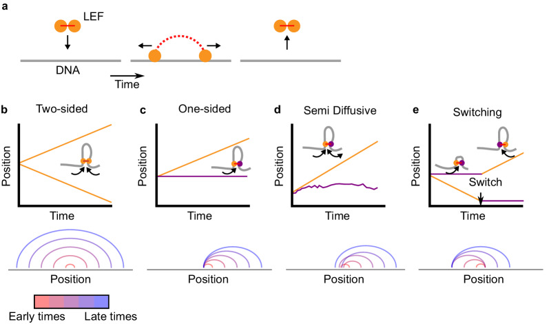
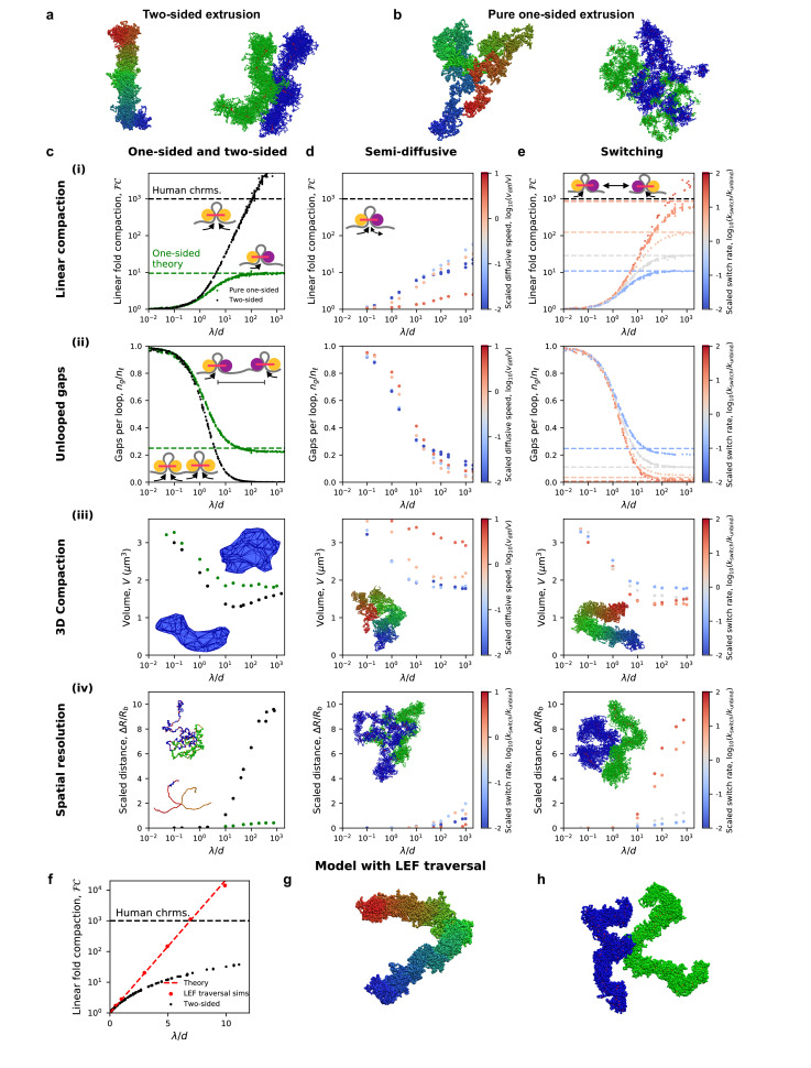
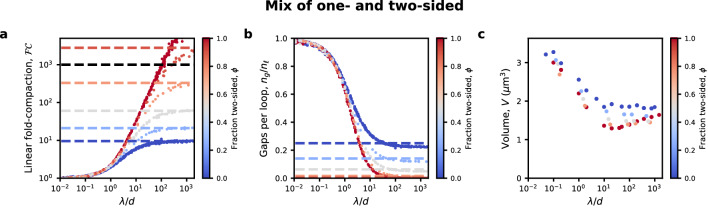
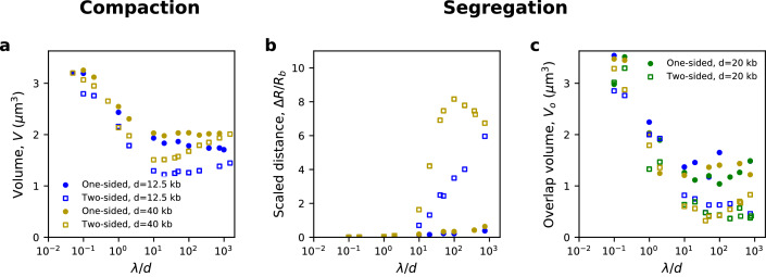
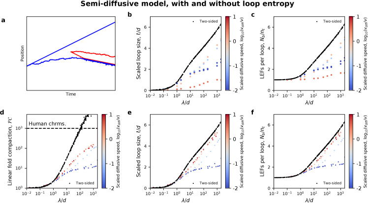
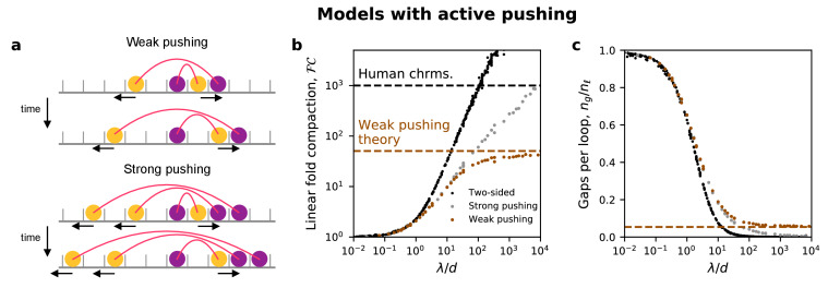
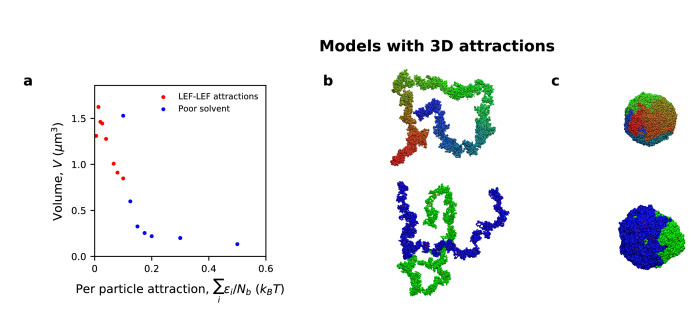
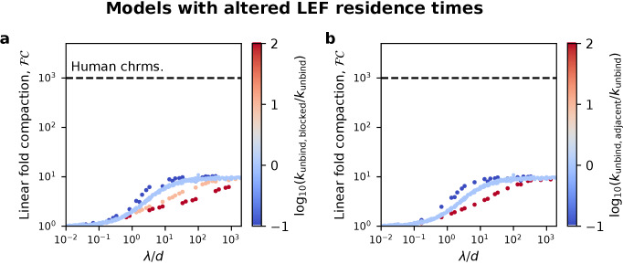
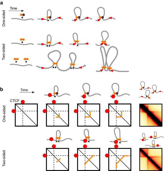
SMC complexes, such as condensin or cohesin, organize chromatin throughout the cell cycle by a process known as loop extrusion. SMC complexes reel in DNA, extruding and progressively growing DNA loops. Modeling assuming two-sided loop extrusion reproduces key features of chromatin organization across different organisms. In vitro single-molecule experiments confirmed that yeast condensins extrude loops, however, they remain anchored to their loading sites and extrude loops in a ‘one-sided’ manner. We therefore simulate one-sided loop extrusion to investigate whether ‘one-sided’ complexes can compact mitotic chromosomes, organize interphase domains, and juxtapose bacterial chromosomal arms, as can be done by ‘two-sided’ loop extruders. While one-sided loop extrusion cannot reproduce these phenomena, variants can recapitulate in vivo observations. We predict that SMC complexes in vivo constitute effectively two-sided motors or exhibit biased loading and propose relevant experiments. Our work suggests that loop extrusion is a viable general mechanism of chromatin organization.
Overview
The claims and statistics of this paper haven’t been checked yet.
Run the check — free, no account needed. It reads the open-access text and checks the sources it cites.
Integrity signals
Registry
Cites
Statistics
Figures
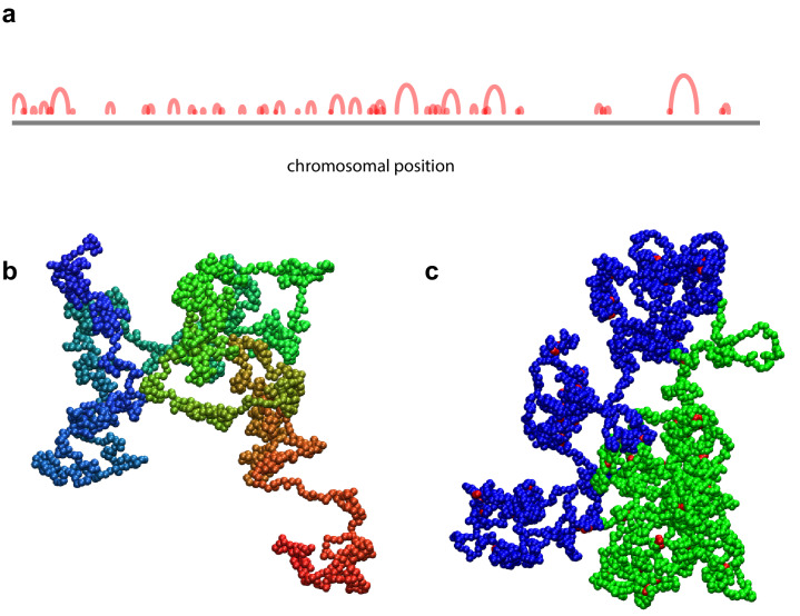
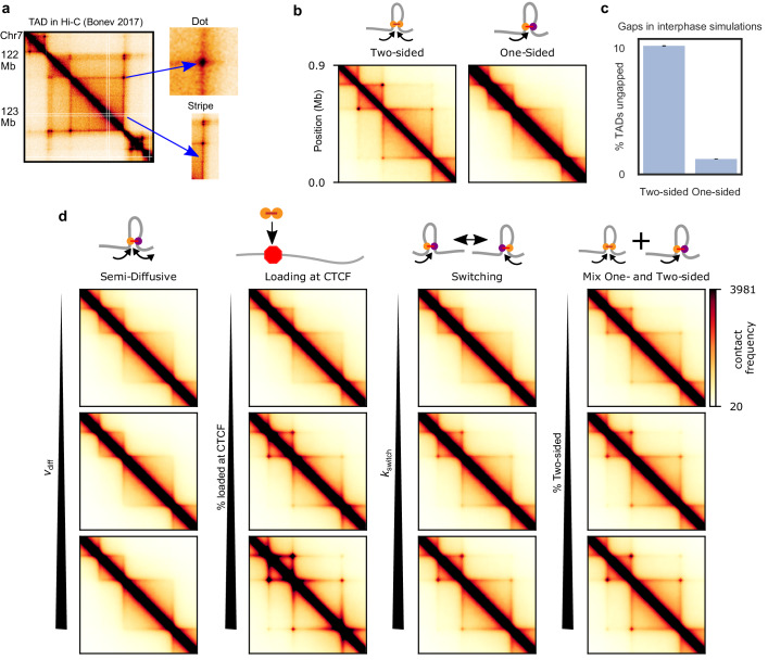
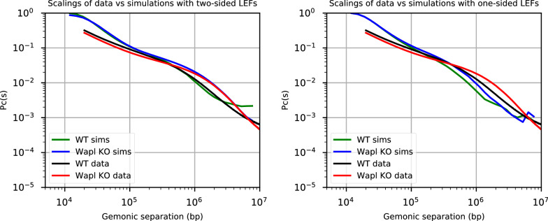
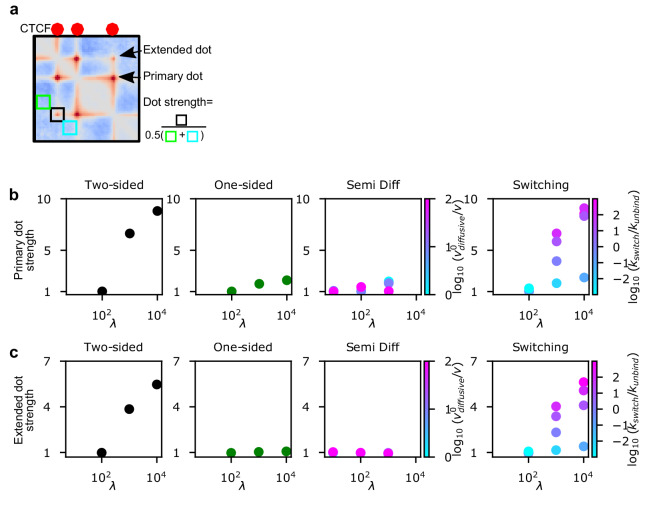
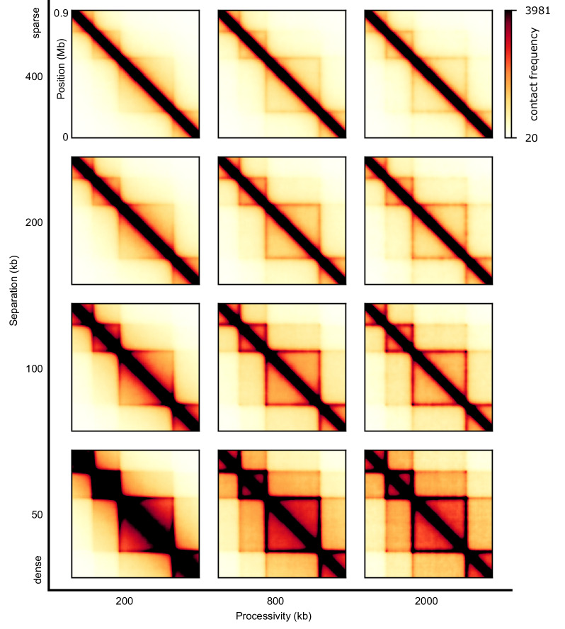
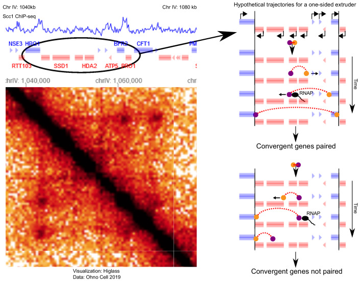
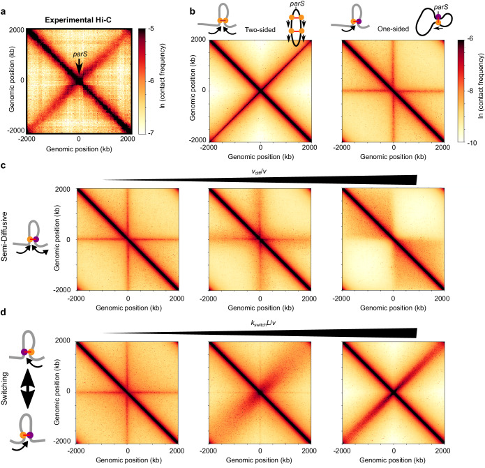
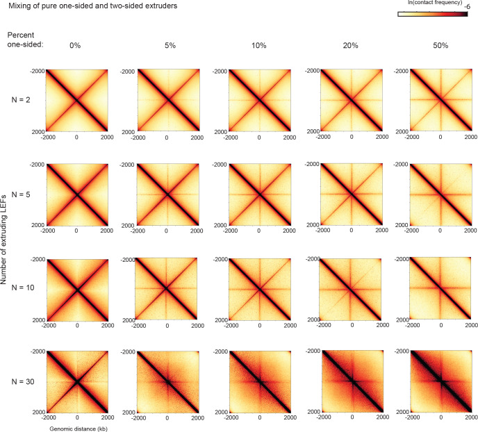
Verification
Claims the paper makes
The claims and statistics of this paper haven’t been checked yet.
Run the check — free, no account needed. It reads the open-access text and checks the sources it cites.
Claims other papers make about this one
Each is checked against this paper’s own text: does it say what the citing paper says it does?
The cited source says what the claim attributes to it.
In the citing paper
“and simulations incorporating two-sided extrusion, rather than one-sided, better reproduce the juxtaposition of bacterial chromosomal arms.78”
From Bringing the genetically minimal cell to life on a computer in 4D (2026) · cites this paper as [78]
Self-check
Percentages, sums and reported differences re-computed from the paper’s own numbers.
The self-check needs the paper’s full text.
Citations
Cites
Exact stochastic simulation of coupled chemical reactions
Gillespie, D. T. (1977) · The Journal of Physical Chemistry · doi:10.1021/j100540a008 · Cited by 10,215 · cited 1×
“We use the Gillespie algorithm to determine the time that each kinetic event -- binding, unbinding, directional stepping, and switching -- occurs (Gillespie, 1977; Goloborodko et al., 2016b).”
MethodA 3D Map of the Human Genome at Kilobase Resolution Reveals Principles of Chromatin Looping
Rao, S. S. P., Huntley, M. H., Durand, N. C., Stamenova, E. K., Bochkov, I. D., Robinson, J. T., Sanborn, A. L., Machol, I., Omer, A. D., Lander, E. S., et al. (2014) · Cell · doi:10.1016/j.cell.2014.11.021 · Cited by 9,212 · cited 8×
“Dots are foci on Hi-C maps that reflect enriched contact frequency between specific loci, often found at the corners of TADs and/or between proximal (<1-2 Mb) CTCF sites (Krietenstein et al., 2019; Rao et al., 2014).”
BackgroundMethodInfluentialComprehensive Mapping of Long-Range Interactions Reveals Folding Principles of the Human Genome
Lieberman-Aiden, E., van Berkum, N. L., Williams, L., Imakaev, M., Ragoczy, T., Telling, A., Amit, I., Lajoie, B. R., Sabo, P. J., Dorschner, M. O., et al. (2009) · Science · doi:10.1126/science.1181369 · Cited by 8,898 · cited 1×
“Dot strengths are computed as follows: first, we compute observed-over-expected of a contact map (we divide out the distance dependence, by dividing each diagonal by its average [Lieberman-Aiden et al., 2009]), then we compute the strength of a dot of a particular TAD (Figure 3—figure supplement 2) and last, we comput…”
MethodSelf-citationTopological domains in mammalian genomes identified by analysis of chromatin interactions
Dixon, J. R., Selvaraj, S., Yue, F., Kim, A., Li, Y., Shen, Y., Hu, M., Liu, J. S., & Ren, B. (2012) · Nature · doi:10.1038/nature11082 · Cited by 6,829
Spatial partitioning of the regulatory landscape of the X-inactivation centre
Nora, E. P., Lajoie, B. R., Schulz, E. G., Giorgetti, L., Okamoto, I., Servant, N., Piolot, T., van Berkum, N. L., Meisig, J., Sedat, J., et al. (2012) · Nature · doi:10.1038/nature11049 · Cited by 2,895
OpenMM 7: Rapid development of high performance algorithms for molecular dynamics
Eastman, P., Swails, J., Chodera, J. D., McGibbon, R. T., Zhao, Y., Beauchamp, K. A., Wang, L.-P., Simmonett, A. C., Harrigan, M. P., Stern, C. D., et al. (2017) · PLOS Computational Biology · doi:10.1371/journal.pcbi.1005659 · Cited by 2,748
Disruptions of Topological Chromatin Domains Cause Pathogenic Rewiring of Gene-Enhancer Interactions
Lupiáñez, D. G., Kraft, K., Heinrich, V., Krawitz, P., Brancati, F., Klopocki, E., Horn, D., Kayserili, H., Opitz, J. M., Laxova, R., et al. (2015) · Cell · doi:10.1016/j.cell.2015.04.004 · Cited by 2,132
Formation of chromosomal domains by loop extrusion
Fudenberg, G., Imakaev, M., Lu, C., Goloborodko, A., Abdennur, N., & Mirny, L. A. (2016) · Cell Reports · doi:10.1016/j.celrep.2016.04.085 · Cited by 2,003
Three-dimensional folding and functional organization principles of the Drosophila genome
Sexton, T., Yaffe, E., Kenigsberg, E., Bantignies, F., Leblanc, B., Hoichman, M., Parrinello, H., Tanay, A., & Cavalli, G. (2012) · Cell · doi:10.1016/j.cell.2012.01.010 · Cited by 1,983
Cohesin Loss Eliminates All Loop Domains
Rao, S. S. P., Huang, S.-C., Glenn St Hilaire, B., Engreitz, J. M., Perez, E. M., Kieffer-Kwon, K.-R., Sanborn, A. L., Johnstone, S. E., Bascom, G. D., Bochkov, I. D., et al. (2017) · Cell · doi:10.1016/j.cell.2017.09.026 · Cited by 1,883
Research works printed but not linked: 5
- de Lange, 1933, Sur un type nouveau de dégénération (typus amstelodamensis), Arch Méd Enfants, 36, 713
- Fytas, 2013, Molecular dynamics simulations of single-component bottle-brush polymers with flexible backbones under poor solvent conditions, Journal of Physics: Condensed Matter, 25, 10.1088/0953-8984/25/28/285105 · DOI
- Glynn, 2004, Genome-wide mapping of the cohesin complex in the yeast Saccharomyces cerevisiae, PLOS Biology, 2, 10.1371/journal.pbio.0020259 · DOI
- Kerpedjiev, 2018, HiGlass: web-based visual exploration and analysis of genome interaction maps, Genome Biology, 19, 10.1186/s13059-018-1486-1 · DOI
- Seitan, 2013, Cohesin-based chromatin interactions enable regulated gene expression within preexisting architectural compartments, Genome Research, 23, 2066, 10.1101/gr.161620.113 · DOI · Paper page
Cited by
Sorted by citations
Transcription shapes 3D chromatin organization by interacting with loop extrusion
Banigan, E. J., Tang, W., van den Berg, A. A., Stocsits, R. R., Wutz, G., Brandão, H. B., Busslinger, G. A., Peters, J., & Mirny, L. A. (2023) · Proceedings of the National Academy of Sciences · doi:10.1073/pnas.2210480120 · Cited by 238
“For active extrusion, τ=100 for CTCF KO and τ=1000 for DKO simulations, giving mean LEF processivities of λ=200 kb and 2000 kb, respectively, similar to previous studies (Banigan et al., 2020; Nuebler et al., 2018).”
BackgroundMethodResultInfluentialSelf-citationCohesin and condensin extrude DNA loops in a cell cycle-dependent manner
Golfier, S., Quail, T., Kimurâ, H., & Jan Brugués, A. (2020) · eLife · doi:10.7554/elife.53885 · Cited by 201
“The cell cycle-dependent activities of con- densin and cohesin could account for the transition between symmetric and non-symmetric loop extrusion (Banigan et al., 2019; Abramo et al., Figure 1 continued https://elifesciences.org/articles/53885#fig1video8 Figure 1—video 9.”
BackgroundResultInfluentialLoop extrusion: theory meets single-molecule experiments
Banigan, E. J., & Mirny, L. A. (2020) · Current Opinion in Cell Biology · doi:10.1016/j.ceb.2020.04.011 · Cited by 169
Self-citationMCM complexes are barriers that restrict cohesin-mediated loop extrusion
Dequeker, B., Scherr, M. J., Brandão, H. B., Gassler, J., Powell, S. T., Gáspár, I., Flyamer, I. M., Lalic, A., Tang, W., Stocsits, R. R., et al. (2020) · Nature · doi:10.1038/s41586-022-04730-0 · Cited by 132
Self-citationLooping the Genome with SMC Complexes
Kim, E., Barth, R., & Dekker, C. (2023) · Annual Review of Biochemistry · doi:10.1146/annurev-biochem-032620-110506 · Cited by 96
CTCF as a boundary factor for cohesin-mediated loop extrusion: evidence for a multi-step mechanism
Hansen, A. S. (2020) · Nucleus · doi:10.1080/19491034.2020.1782024 · Cited by 101
“Polymer simulations of the simple loop extrusion model with just cohesin and CTCF generate contact maps similar to experimental maps at the level of TADs and loop domains [17,18,38,44,77].”
MethodDNA-loop-extruding SMC complexes can traverse one another in vivo
Brandão, H. B., Ren, Z., Karaboja, X., Mirny, L. A., & Wang, X. (2021) · Nature Structural & Molecular Biology · doi:10.1038/s41594-021-00626-1 · Cited by 90
“In eukaryotes, bypassing can help promote chromosome compaction and sister-chromatid segregation 30,36 .”
BackgroundMethodInfluentialSelf-citationChromatin architecture transitions from zebrafish sperm through early embryogenesisPreprint
Wike, C. L., Guo, Y., Tan, M., Nakamura, R., Shaw, D. K., Díaz, N., Whittaker-Tademy, A. F., Durand, N. C., Aiden, E. L., Vaquerizas, J. M., et al. (2021) · Genome Research · doi:10.1101/gr.269860.120 · Cited by 87
Tracking and interpreting long-range chromatin interactions with super-resolution live-cell imaging
Brandão, H. B., Gabriele, M., & Hansen, A. S. (2021) · Current Opinion in Cell Biology · doi:10.1016/j.ceb.2020.11.002 · Cited by 77
Self-citationChromatin jets define the properties of cohesin-driven in vivo loop extrusion.
Guo, Y., Al-Jibury, E., Garcia-Millan, R., Ntagiantas, K., King, J. W. D., Nash, A. J., Galjart, N., Lenhard, B., Rueckert, D., Fisher, A., et al. (2022) · Molecules and Cells · doi:10.1016/j.molcel.2022.09.003 · Cited by 69
Spatial Organization of Chromatin: Emergence of Chromatin Structure During Development
Ghosh, R. P., & Meyer, B. J. (2021) · Annual Review of Cell and Developmental Biology · doi:10.1146/annurev-cellbio-032321-035734 · Cited by 60
“Polymer simulations showed that stochastic strand switching can efficiently recapitulate chromosome compaction levels achieved through a two-sided extrusion model (Banigan et al. 2020) (Figure 1c–f).”
BackgroundVos, E. S. M., Valdes‐Quezada, C., Huang, Y., Allahyar, A., Verstegen, M. J. A. M., Felder, A.-K., van der Vegt, F., Uijttewaal, E. C. H., Krijger, P. H. L., & de Laat, W. L. (2021) · Molecular Cell · doi:10.1016/j.molcel.2021.06.008 · Cited by 61
Nomidis, S. K., Carlon, E., Gruber, S., & Marko, J. (2022) · bioRxiv · doi:10.1093/nar/gkac268 · Cited by 48
Self-citationSuper-Enhancers, Phase-Separated Condensates, and 3D Genome Organization in Cancer
Tang, S. C., Vijayakumar, U., Zhang, Y., & Fullwood, M. J. (2022) · Cancers · doi:10.3390/cancers14122866 · Cited by 56
“This is explained by the loop extrusion model in which frequent transient loops are organised by structural maintenance of chromosomes (SMC) complexes that reel in chromatin, forming growing loops that stop at CCCTC-binding factor (CTCF) boundaries [14,15].”
BackgroundSMC complexes: Lifting the lid on loop extrusion
Higashi, T. L., & Uhlmann, F. (2022) · Current Opinion in Cell Biology · doi:10.1016/j.ceb.2021.12.003 · Cited by 58
Bringing the genetically minimal cell to life on a computer in 4D
Thornburg, Z. R., Maytin, A., Kwon, J., Brier, T. A., Gilbert, B. R., Fu, E., Gao, Y.-L., Quenneville, J., Wu, T., Li, H., et al. (2026) · Cell · doi:10.1016/j.cell.2026.02.009 · Cited by 44
SMC motor proteins extrude DNA asymmetrically and can switch directions
Barth, R., Davidson, I. F., van der Torre, J., Taschner, M., Gruber, S., Peters, J.-M., & Dekker, C. (2025) · Cell · doi:10.1016/j.cell.2024.12.020 · Cited by 40
“Close inspection of their loop extrusion dynamics revealed that cohesin and SMC5/6 undergo short phases of active extrusion, characterized by loop growth, which are interspersed by diffusion 3 of the loop and SMC across the DNA, and loop slipping, the gradual loss of the previously extruded loop.”
InfluentialCondensin DC loads and spreads from recruitment sites to create loop-anchored TADs in C. elegans
Kim, J., Jimenez, D., Ragipani, B., Zhang, B., Street, L., Kramer, M., Albritton, S., Winterkorn, L., Morao, A., & Ercan, S. (2022) · bioRxiv · doi:10.1101/2021.03.23.436694 · Cited by 38
“As randomly distributed LEFs track along DNA, pairs of increasingly distant genomic loci are looped in 3-dimensional space except when LEFs encounter a barrier.”
BackgroundInfluentialPredicting Genome Architecture: Challenges and Solutions
Belokopytova, P. S., & Fishman, V. (2021) · Frontiers in Genetics · doi:10.3389/fgene.2020.617202 · Cited by 36
“A recent preprint from Banigan et al. (2020) shows another impressive application of polymer modeling in which it helps to investigate if a one-or two-sided loop extrusion model works in the cell and to identify a class of one-sided extrusion models that can reproduce in vivo experiments.”
BackgroundStefano, M. D., Paulsen, J., Jost, D., & Martı́-Renom, M. A. (2020) · Current Opinion in Genetics & Development · doi:10.1016/j.gde.2020.10.004 · Cited by 44
Extrusion fountains are hallmarks of chromosome organization emerging upon zygotic genome activation
Galitsyna, A. A., Ulianov, S. V., Bazarevich, M., Bykov, N. S., Veil, M., Gao, M., Perevoschikova, K., Gelfand, M. S., Razin, S. V., Mirny, L. A., et al. (2026) · Nature Communications · doi:10.1038/s41467-026-69105-9 · Cited by 42
Self-citationDNA double-strand break end synapsis by DNA loop extrusion
Yang, J. H., Brandão, H. B., & Hansen, A. S. (2023) · Nature Communications · doi:10.1038/s41467-023-37583-w · Cited by 36
Self-citationLocal chromatin fiber folding represses transcription and loop extrusion in quiescent cells
Swygert, S. G., Lin, D., Portillo‐Ledesma, S., Lin, P.-Y., Hunt, D. R., Kao, C.-F., Tamar Schlick, A., Noble, W. S., & Tsukiyama, T. (2021) · eLife · doi:10.7554/elife.72062 · Cited by 48
Rapid depletion of CTCF and cohesin proteins reveals dynamic features of chromosome architecturePreprint
Liu, N.-Q., Magnitov, M. D., Schijns, M. M. G. A., van Schaik, T., van der Weide, R. H., Teunissen, H., van Steensel, B., & de Wit, E. (2021) · bioRxiv · doi:10.1101/2021.08.27.457977 · Cited by 34
“In Bacillus subtilis, SMC complexes, which are related to cohesin, can be coordinately loaded at the origin of replication using a temperature sensitive mutant (Banigan et al., 2020; Wang et al., 2017, 2018).”
BackgroundCohesin organizes 3D DNA contacts surrounding active enhancers in C. elegansPreprint
Kim, J., Wang, H., & Ercan, S. (2025) · Genome Research · doi:10.1101/gr.279365.124 · Cited by 31
“In simulation, cohesin was inferred to be an effectively two-sided loop-extruding factor (Banigan et al. 2020).”
A comparison of topologically associating domain callers over mammals at high resolution
Sefer, E. (2022) · BMC Bioinformatics · doi:10.1186/s12859-022-04674-2 · Cited by 37
“The loop extrusion is thought to be a viable chromatin organization mechanism according to [48, 102].”
BackgroundChan, B., & Rubinstein, M. (2024) · Proceedings of the National Academy of Sciences · doi:10.1073/pnas.2401494121 · Cited by 34
“Compaction on longer contour length scales extends within topologically associated domains (TADs), facilitating gene regulation by distal elements.”
Liu, Y., Zhao, N., Kanemaki, M. T., Yamamoto, Y., Sadamura, Y., Ito, Y., Tokunaga, M., Stasevich, T. J., & Kimurâ, H. (2021) · Genes to Cells · doi:10.1111/gtc.12893 · Cited by 29
“First, the ZF target sequence should be within 10 kb from the chromatin contact sites considering the resolution of light microscopy (Banigan et al., 2020; Brandão et al., 2021).”
A Lamin Associated Chromatin Model for Chromosome Organization
Maji, A., Ahmed, J., Roy, S., Chakrabarti, B., & Mitra, M. K. (2019) · bioRxiv · doi:10.1101/788497 · Cited by 28
Loop extrusion rules: the next generation.
Corsi, F., Rusch, E., & Goloborodko, A. (2023) · Current Opinion in Genetics and Development · doi:10.1016/j.gde.2023.102061 · Cited by 27
Nanoscale DNA tracing reveals the self-organization mechanism of mitotic chromosomes
Beckwith, K. S., Brunner, A. H., Morero, N. R., Jungmann, R., & Ellenberg, J. (2025) · Cell · doi:10.1016/j.cell.2025.02.028 · Cited by 27
“41,42 Both one-and two-sided extrusion modes have been reported for human condensin.”
All eukaryotic SMC proteins induce a twist of −0.6 at each DNA loop extrusion step
Janissen, R., Barth, R., Davidson, I., Taschner, M., Gruber, S., Peters, J.-M., & Dekker, C. (2024) · bioRxiv · doi:10.1126/sciadv.adt1832 · Cited by 26
“…contribute to the appearance of characteristic CTCF-dependent TAD corner dots in high-throughput chromosome conformation capture (Hi-C) maps ( 59 , 74 , 75 ) since those depend on a fraction of TADs whose DNA is completely contained in SMC-mediated loops ( 76 ) as observed in vivo ( 77 , 78 ).”
Extrusion fountains are restricted by WAPL-dependent cohesin release and CTCF barriers
Liu, N. Q., Magnitov, M. D., Schijns, M. M. G. A., van Schaik, T., Teunissen, H., van Steensel, B., & de Wit, E. (2025) · Nucleic Acids Research · doi:10.1093/nar/gkaf549 · Cited by 33
Predicting genome organisation and function with mechanistic modelling
Chiang, M., Brackley, C. A., Marenduzzo, D., & Gilbert, N. (2021) · Trends in Genetics · doi:10.1016/j.tig.2021.11.001 · Cited by 35
“This finding led to more theoretical work examining the impact of one-sided versus two-sided extrusion on the resulting domain architecture [54,55].”
Bendandi, A., Dante, S., Zia, S. R., Diaspro, A., & Rocchia, W. (2020) · Frontiers in Molecular Biosciences · doi:10.3389/fmolb.2020.00015 · Cited by 23
“In addition to the “one-sided” loop extrusion mechanism described above, recent research indicates that “two-sided” loop extrusion might prove to be more robust in explaining experimental data (Banigan et al., 2019).”
BackgroundGenome-wide absolute quantification of chromatin looping
Jusuf, J. M., Yang, J. H., Toppen, J., Grosse-Holz, S., Gabriele, M., Mach, P., Flyamer, I. M., Zechner, C., Giorgetti, L., Mirny, L. A., et al. (2026) · Nature Structural & Molecular Biology · doi:10.1038/s41594-026-01819-2 · Cited by 22
Self-citationFunction and Evolution of the Loop Extrusion Machinery in Animals
Kabirova, E., Nurislamov, A. R., Shadskiy, A., Smirnov, A. V., Popov, A., Salnikov, P., Баттулин, Н. Р., & Fishman, V. (2023) · International Journal of Molecular Sciences · doi:10.3390/ijms24055017 · Cited by 27
“The other one, one-sided loop extrusion, suggests that a fraction of SMC complexes reel in DNA from only one side, while the other side remains anchored to its DNA loading site [30].”
BackgroundNicE-C efficiently reveals open chromatin–associated chromosome interactions at high resolutionPreprint
Luo, Z.-Y., Zhang, R., Hu, T.-F., Zhu, Y.-T., Wu, Y.-M., Li, W.-F., Zhang, Z., Yao, X.-B., Liang, H.-Y., & Song, X.-Y. (2022) · Genome Research · doi:10.1101/gr.275986.121 · Cited by 20
“A stripe emerges when one side of extruding is stalled by CTCF while the other side continues extruding (Banigan et al. 2020).”
BackgroundDynamics of chromosome organization in a minimal bacterial cell
Gilbert, B. R., Thornburg, Z. R., Brier, T. A., Stevens, J. A., Grünewald, F., Stone, J. E., Marrink, S. J., & Luthey-Schulten, Z. (2023) · Frontiers in Cell and Developmental Biology · doi:10.3389/fcell.2023.1214962 · Cited by 19
“…Giorgetti, 2019) are required to solve the inverse problem of determining 3D genome organization (Di Pierro et al., 2017; Messelink et al., 2021; Shi and Thirumalai, 2023) and provide mechanistic insights (Sanborn et al., 2015; Fudenberg et al., 2016; Banigan et al., 2020; Fiorillo et al., 2021).”
A low Smc flux avoids collisions and facilitates chromosome organization in Bacillus subtilis
Anchimiuk, A., Lioy, V., Bock, F., Minnen, A., Boccard, F., & Gruber, S. (2021) · eLife · doi:10.7554/elife.65467 · Cited by 19
“undesirable DNA entanglements (such as pseudoknots) (Banigan et al., 2020).”
Decoding the organization, dynamics, and function of the 4D genome
Aboelnour, E., & Bonev, B. (2021) · Developmental Cell · doi:10.1016/j.devcel.2021.04.023 · Cited by 24
The interplay between asymmetric and symmetric DNA loop extrusion
Banigan, E., & Mirny, L. (2020) · bioRxiv · doi:10.7554/elife.63528 · Cited by 19
Self-citationMatityahu, A., & Onn, I. (2021) · Journal of Cell Science · doi:10.1242/jcs.247577 · Cited by 22
“Loop extrusion suppression in condensin and Smc5/6 Loop extrusion is also considered a component of the mitotic chromosome assembly mechanism by the cohesin-related SMC complex condensin (Banigan et al., 2020; Ganji et al., 2018; Kim et al., 2020; Terakawa et al., 2017).”
BackgroundFob1-dependent condensin recruitment and loop extrusion on yeast chromosome III
Dinda, M., Fine, R. D., Saha, S., Wang, Z., Zang, C., Li, M., & Smith, J. S. (2022) · bioRxiv · doi:10.1371/journal.pgen.1010705 · Cited by 15
Loops and the activity of loop extrusion factors constrain chromatin dynamics
Bailey, M. L. P., Surovtsev, I. V., Williams, J. F., Yan, H., Yuan, T., Li, K., Duseau, K., Mochrie, S. G. J., & King, M. C. (2023) · Molecular Biology of the Cell · doi:10.1091/mbc.e23-04-0119 · Cited by 22
“LEF simulations further demonstrate that the dynamic extrusion of loops by SMC complexes combined with the existence of boundary elements encoded in the DNA (for example, sequence-specific binding of CTCF, which is enriched at boundaries and physically interacts with cohesin (Parelho et al., 2008; Wendt et al., 2008))…”
BackgroundInfluentialDynamics of microcompartment formation at the mitosis-to-G1 transition
Goel, V. Y., Aboreden, N. G., Jusuf, J. M., Zhang, H., Mori, L., Mirny, L. A., Blobel, G. A., Banigan, E. J., & Hansen, A. S. (2025) · Nature Structural & Molecular Biology · doi:10.1038/s41594-025-01687-2 · Cited by 35
“6a, top) 37,48–50 .”
Self-citationDNA packaging by molecular motors: from bacteriophage to human chromosomes
Prevo, B., & Earnshaw, W. C. (2024) · Nature Reviews Genetics · doi:10.1038/s41576-024-00740-y · Cited by 11
“This ‘switching model’ was found to be the only one-sided extruder model capable of achieving proper chromosome compaction 137 .”
SMC motor proteins extrude DNA asymmetrically and contain a direction switchPreprint
Barth, R., Davidson, I., van der Torre, J., Taschner, M., Gruber, S., Peters, J.-M., & Dekker, C. (2023) · bioRxiv · doi:10.1101/2023.12.21.572892 · Cited by 14
“…the experimentally observed interphase chromosome organization, in particular the formation of TADs, even if the anchor site is only diffusively bound to DNA 56 , while asymmetric extrusion with Z-loop formation and direction switching could recapitulate mitotic chromosome formation 56,57 .”
BackgroundMoDLE: high-performance stochastic modeling of DNA loop extrusion interactions
Rossini, R., Kumar, V., Mathelier, A., Rognes, T., & Paulsen, J. (2022) · bioRxiv · doi:10.1186/s13059-022-02815-7 · Cited by 14
“assessed the level of DNA compaction that can be achieved by different loop extrusion mechanisms and concluded that one-sided loop extrusion alone fails to achieve the level of compaction observed in large metazoan genomes [36].”
BackgroundMethodDrosophila insulator proteins exhibit in vivo liquid–liquid phase separation properties
Amankwaa, B., Schoborg, T. A., & Labrador, M. (2022) · Life Science Alliance · doi:10.26508/lsa.202201536 · Cited by 19
“Insulator and cohesin proteins synergistically mediate the formation of TADs through a chromatin looping process known as loop extrusion in mammals (8, 9).”
BackgroundMultiple parameters shape the 3D chromatin structure of single nuclei at the doc locus in Drosophila
Götz, M., Messina, O., Espínola, S., Fiche, J.-B., & Nöllmann, M. (2022) · Nature Communications · doi:10.1038/s41467-022-32973-y · Cited by 16
“In contrast, chromatin behaves as a random-coil polymer in the absence of cohesin or in absence of monomer-monomer interactions 40,63,64 .”
Polymer simulations guide the detection and quantification of chromatin loop extrusion by imaging
Sabaté, T., Lelandais, B., Bertrand, E., & Zimmer, C. (2023) · Nucleic Acids Research · doi:10.1093/nar/gkad034 · Cited by 13
“To model loop extrusion, we assumed that a single loop extrusion complex was loaded on the polymer at a random position between the two anchors, whereafter both sides of the polymer chain were extruded simultaneously (bidirectional extrusion (26,71)).”
Vinayak, V., Basir, R., Golloshi, R., Toth, J. M., Sant’Anna, L. E., Lakadamyali, M., McCord, R. P., & Shenoy, V. B. (2025) · Nature Communications · doi:10.1038/s41467-025-59001-z · Cited by 9
“…approaches have provided insight into the dynamic reorganization of chromatin during the transition from interphase to mitosis 101 , revealing the crucial roles of looping motors 48 and transcription-driven supercoiling dynamics in chromatin compaction and recon fi guration 11,102,103 .”
The “Genomic Code”: DNA Pervasively Moulds Chromatin Structures Leaving no Room for “Junk”
Bernardi, G. (2021) · Life · doi:10.3390/life11040342 · Cited by 14
“Extrusion has, however, several problems: (1) removal of cohesin and CTCF from chromosomes showed limited effects on steady-state transcription [85–87]; (2) extrusion does not appear to be a general phenomenon in chromatin domains; indeed, it is “malleable and variable between individual cells” [88] and absent in Dros…”
BackgroundZabolotnaya, E., Mela, I., Henderson, R. M., & Robinson, N. P. (2020) · Biochemical Society Transactions · doi:10.1042/bst20170168 · Cited by 12
Two CTCF motifs impede cohesin-mediated DNA loop extrusion
Barth, R., Janissen, R., Muras, L., van der Torre, J., Litos, G., van der Sluis, E. O., van den Berg, A., Davidson, I., Peters, J.-M., & Dekker, C. (2025) · bioRxiv · doi:10.1101/2025.01.26.634934 · Cited by 12
“…to what extent stalling of cohesin, rather than direction reversal, can explain Hi-C maps, we performed 3D polymer simulations (STAR Methods), 69,70 varying two key parameters: (1) the probability of CTCF stalling cohesin and (2) the likelihood that this stalling also prevents extrusion away…”
Comparative study on chromatin loop callers using Hi-C data reveals their effectiveness
Chowdhury, H. M. A. M., Boult, T. E., & Oluwadare, O. (2023) · bioRxiv · doi:10.1186/s12859-024-05713-w · Cited by 12
“These loops and peaks are important regions from which we can answer questions about chromatin interaction and conformation [6, 9].”
BackgroundAbdulla, A. Z., Salari, H., Tortora, M. M. C., Vaillant, C., & Jost, D. (2023) · Current Opinion in Genetics & Development · doi:10.1016/j.gde.2023.102033 · Cited by 16
Yin, S., NandyMazumdar, M., Paranjapye, A., & Harris, A. (2022) · Genomics · doi:10.1016/j.ygeno.2022.110350 · Cited by 13
Câmara, A. S., Schubert, V., Mascher, M., & Houben, A. (2021) · bioRxiv · doi:10.1093/nar/gkab648 · Cited by 12
“We adopted two-sided LEs because (34) showed that one-sided LEs could not reproduce alone some biological phenomena.”
MethodRNA polymerase backtracking results in the accumulation of fission yeast condensin at active genes
Rivosecchi, J., Jost, D., Vachez, L., Gautier, F. D., Bernard, P., & Vanoosthuyse, V. (2021) · Life Science Alliance · doi:10.26508/lsa.202101046 · Cited by 20
“An inability to bypass obstacles might result in the formation of unlooped chromatin gaps within mitotic chromosomes (Banigan et al, 2020).”
Rusková, R., & Račko, D. (2021) · Biology · doi:10.3390/biology10020130 · Cited by 12
“Today, the role of SMCs in loop formation and chromosome organization in organisms from bacteria to humans is generally accepted [11].”
BackgroundMaji, A., Padinhateeri, R., & Mitra, M. K. (2019) · bioRxiv · doi:10.1101/861161 · Cited by 12
The physical chemistry of interphase loop extrusion
Tortora, M. M. C., & Fudenberg, G. (2024) · bioRxiv · doi:10.1101/2024.08.23.609419 · Cited by 11
“…et al., 2023) , a dependence of the loop extrusion rate on chromatin tension (Nomidis et al., 2022) and/or local conformation (Conforto et al., 2024) , cohesin backtracking and bypassing (Banigan and Mirny, 2020) or capture of spatially proximal chromatin in trans (Bonato and Michieletto, 2021) .”
Meiotic chromosome organization and crossover patterns
Shang, Y.-L., Tan, T.-C., Fan, C., Nie, H., Wang, Y., Yang, X., Zhai, B., Wang, S., & Zhang, L.-R. (2022) · Biology of Reproduction · doi:10.1093/biolre/ioac040 · Cited by 11
Seeing the forest through the trees: prioritising potentially functional interactions from Hi-C
Liu, N., Low, W. Y., Alinejad‐Rokny, H., Pederson, S., Sadlon, T. J., Barry, S. C., & Breen, J. (2021) · Epigenetics & Chromatin · doi:10.1186/s13072-021-00417-4 · Cited by 16
Cohesin and condensin extrude loops in a cell-cycle dependent manner
Golfier, S., Quail, T., Kimura, H., & Brugués, J. (2019) · bioRxiv · doi:10.1101/821306 · Cited by 10
Chromosomal domain formation by archaeal SMC, a roadblock protein, and DNA structure
(2025) · doi:10.1038/s41467-025-56197-y · Cited by 10
“A simulation study showed that, if a loop-extruding factor shapes a boundary at its loading site as postulated above, it must perform asymmetric loop extrusion combined with one-dimensional diffusion along DNA 83 .”
LoopSage: An Energy-Based Monte Carlo approach for the Loop Extrusion Modelling of Chromatin
Korsak, S., & Plewczynski, D. (2024) · bioRxiv · doi:10.1101/2024.01.10.574968 · Cited by 9
“…how loop extrusion impacts chromatin folding and the global chromatin structure, examining the effects of different types of LE (one-sided, two-sided, symmetrical, asymmetrical) [16, 18, 20] and exploring the influence of other protein remodelers, such as RNApII, on cohesin dynamics [21–24].”
BackgroundMolecular dynamics simulations for the study of chromatin biology
Brandani, G. B., Gopi, S., Yamauchi, M., & Takada, S. (2022) · Current Opinion in Structural Biology · doi:10.1016/j.sbi.2022.102485 · Cited by 16
Landscape of the Epstein-Barr virus-host chromatin interactome and gene regulation
Tian, S., Yang, Y., Ning, D., Yu, T., Gao, T., Deng, Y., Fang, K., Xu, Y., Jing, K., Huang, G., et al. (2025) · EMBO Journal · doi:10.1038/s44318-025-00466-5 · Cited by 8
“5P), differing from the asymmetric DNA loop extrusion commonly driven by RNAPII or CTCF (Banigan et al, 2020; Zheng et al, 2019).”
Interactions Between Nucleosomes: From Atomistic Simulation to Polymer Model
Zhang, C., & Huang, J. (2021) · Frontiers in Molecular Biosciences · doi:10.3389/fmolb.2021.624679 · Cited by 8
“, 2016), and shed light on the mechanisms underlying the folding and organization of chromatin (Gibcus et al., 2018; Mirny et al., 2019; Stam et al., 2019; Banigan et al., 2020).”
BackgroundLocus architecture and RAG scanning determine antibody diversity
Kenter, A., Priyadarshi, S., & Drake, E. B. (2023) · Trends in immunology · doi:10.1016/j.it.2022.12.005 · Cited by 7
Belan, S., & Parfenyev, V. (2024) · The Journal of Chemical Physics · doi:10.1063/5.0199573 · Cited by 8
Keeping intracellular DNA untangled: A new role for condensin?
Roca, J., Dyson, S., Segura, J., Valdés, A., & Martínez-García, B. (2021) · Bioessays · doi:10.1002/bies.202100187 · Cited by 7
PDS5 proteins control genome architecture by limiting the lifetime of cohesin-NIPBL complexes
Wutz, G., Davidson, I. F., Banigan, E. J., Stocsits, R. R., Kawasumi, R., Tang, W., Nagasaka, K., Costantino, L., Jansen, R., Hirota, K., et al. (2026) · Molecular Cell · doi:10.1016/j.molcel.2026.03.025 · Cited by 12
Self-citationReplisomes restrict SMC translocation in vivo
Liao, Q., Brandão, H. B., Ren, Z., & Wang, X.-D. (2025) · Nature Communications · doi:10.1038/s41467-025-62596-y · Cited by 6
“1 dynamics, we adapted a framework based on previous measurements and simulations 37,39,45 and included parameters speci fi c to this study (see details in Supplementary Methods).”
Self-citationWang, J., Cheng, K.-K., Yan, C.-K., Luo, H., & Luo, J.-W. (2025) · BMC Bioinformatics · doi:10.1186/s12859-025-06092-6 · Cited by 6
Dynamical properties of chromatin provide insights into key folding principles
Kadam, S., Sahoo, S., Kumar, P. B. S., & Padinhateeri, R. (2025) · bioRxiv · doi:10.1101/2024.05.07.592992 · Cited by 5
Loop-extruder mediated rigidity can globally order bacterial chromosomes
Harju, J., Armbruster, T., & Broedersz, C. P. (2024) · bioRxiv · doi:10.1101/2024.10.10.617531 · Cited by 5
“To develop a computational model for our system, we adapt a previously used simulation scheme [42], where 1D simulations of loop extrusion are used to dynamically constrain 3D polymer simulations.”
Yuan, T., Yan, H., Li, K., Surovtsev, I. V., King, M. C., & Mochrie, S. G. J. (2024) · Genome biology · doi:10.1186/s13059-024-03432-2 · Cited by 7
Buka, K., Parteka-Tojek, Z., Agarwal, A., Denkiewicz, M., Korsak, S., Chiliński, M., Banecki, K. H., & Plewczyński, D. (2025) · Communications Biology · doi:10.1038/s42003-025-07847-w · Cited by 4
“…loop extrusion process for an exemplary region on chromosome 1 ( Figure 3C ), Usually, to simulate loop extrusion, stochastic models are used (16, 28, 48–50), where the cohesin proteins on the chromatin fibre perform one-dimensional random walk motion, and they may unload or load in different…”
Spectral-based detection of chromatin loops in multiplexed super-resolution FISH data
Liefsoens, M., Földes, T., & Barbi, M. (2024) · Nature Communications · doi:10.1038/s41467-024-51650-w · Cited by 6
“As insulator proteins, CTCF and cohesin regulate chromatin loop stability, probably as a ’ dynamic complex ’ that frequently breaks and reforms throughout the cell cycle 12 .”
StripeDiff: Model-based algorithm for differential analysis of chromatin stripe
Gupta, K., Wang, G., Zhang, S., Gao, X.-L., Zheng, R., Zhang, Y., Meng, Q., Zhang, L.-L., Cao, Q., & Chen, K.-F. (2022) · Science Advances · doi:10.1126/sciadv.abk2246 · Cited by 4
DNA sliding and loop formation by E. coli SMC complex: MukBEF
Zhou, M. (2021) · bioRxiv · doi:10.1016/j.bbrep.2022.101297 · Cited by 4
Starkov, D., Parfenyev, V., & Belan, S. (2021) · Journal of Chemical Physics · doi:10.1063/5.0048942 · Cited by 4
Exploring the energy landscape of bacterial chromosome segregation
Brahmachari, S., Oliveira, A. B., Mello, M. F., Contessoto, V. G., & Onuchic, J. (2026) · bioRxiv · doi:10.1101/2024.07.27.604869 · Cited by 3
DNA actively regulates the “safety-belt” dynamics of condensin during loop extrusion
Chen, J., Feng, C., Wang, Y., & Chu, X. (2026) · Nature Communications · doi:10.1038/s41467-025-68239-6 · Cited by 3
“6 as the optimal interaction strength between DNA and Ycg1 (see Methods for details).”
InfluentialIrvin, E. M., & Wang, H. (2023) · DNA repair · doi:10.1016/j.dnarep.2023.103528 · Cited by 4
Franek, M., Kilar, A. M., Fojtík, P., Olšinová, M., Benda, A., Rotrekl, V., Dvořáčková, M., & Fajkus, J. (2021) · Journal of Cell Science · doi:10.1242/jcs.258374 · Cited by 3
Fine-tuning of the Smc flux facilitates chromosome organization in B. subtilis
Anchimiuk, A., Lioy, V., Minnen, A., Boccard, F., & Gruber, S. (2020) · bioRxiv · doi:10.1101/2020.12.04.411900 · Cited by 3
Chromatin Fiber Folding Represses Transcription and Loop Extrusion in Quiescent Cells
Swygert, S. G., Lin, D., Portillo-Ledesma, S., Lin, P.-Y., Hunt, D. R., Kao, C., Schlick, T., Noble, W. S., & Tsukiyama, T. (2020) · bioRxiv · doi:10.1101/2020.11.24.396713 · Cited by 3
RNA polymerase backtracking drives the accumulation of fission yeast condensin at active genes
Rivosecchi, J., Vachez, L., Gautier, F., Bernard, P., & Vanoosthuyse, V. (2020) · bioRxiv · doi:10.1101/2020.11.13.381434 · Cited by 3
A comparative analysis of topological domain callers over RNA-associated interactome
Alaygut, T., & Sefer, E. (2026) · BMC Bioinformatics · doi:10.1186/s12859-026-06432-0 · Cited by 2
“Loop extrusion is regarded as a likely mechanism for chromatin organization within DNA domains, according to studies such as [96, 100].”
The physical chemistry of interphase loop extrusion
Tortora, M. M. C., & Fudenberg, G. (2025) · Cell Genomics · doi:10.1016/j.xgen.2025.101098 · Cited by 9
“Many alternatives and elaborations are likely, including asymmetric extrusion with switching, 40,69 a dependence of the loop-extru-sion rate on local conformation, 70 cohesin backtracking and by-passing, 71 or capture of spatially proximal chromatin in trans .”
Zhegalova, I., Ulianov, S., Galitsyna, A., Pletenev, I., Tsoy, O., Luzhin, A. V., Vasiluev, P., Bulavko, E. S., Ivankov, D., Gavrilov, A., et al. (2024) · bioRxiv · doi:10.1101/2024.06.12.598618 · Cited by 2
“This is likely caused by the high density of TSSs: 72, 51, 11, and 1 TSSs per 100 kb on average for Dicty, budding yeast, fruit fly, and human cells, respectively.”
BackgroundNature of barriers determines first passage times in heterogeneous media.
Dasgupta, M., Guha, S., Armbruster, L., Das, D., & Mitra, M. K. (2022) · Soft Matter · doi:10.1039/d4sm00908h · Cited by 2
Osadská, M., Selicky, T., Kretová, M., Jurcik, J., Sivakova, B., Cipakova, I., & Cipak, L. (2022) · International Journal of Molecular Sciences · doi:10.3390/ijms23073939 · Cited by 2
Chromatin dynamics are constrained by loops and driven by the INO80 nucleosome remodelerPreprint
Bailey, M. L. P., Surovtsev, I., Williams, J. F., Yan, H., Yuan, T.-Y., Mochrie, S., & King, M. (2020) · bioRxiv (Cold Spring Harbor Laboratory) · doi:10.1101/2020.02.29.969683 · Cited by 2
D'Asaro, D., Arbona, J., Vaillant, C., & Jost, D. (2026) · bioRxiv · doi:10.1093/nar/gkag731 · Cited by 1
“Note that our model for loop extrusion is minimal and does not account for extra processes, such as stalling at and by-passing barriers that may lead to slight corrections to our predictions [ 57 , 59 , 60 ].”
Metadata
- Authors
- Banigan, E. J., van den Berg, A. A., Brandão, H. B., Marko, J. F., & Mirny, L. A.
- Affiliations
- Massachusetts Institute of Technology (US)
- Harvard University (US)
- Northwestern University (US)
- Corresponding author
- Mirny, Leonid A
- Venue
- eLife
- Publisher
- eLife Sciences Publications, Ltd
- Published
- 2020-04-06
- Volume
- 9
- ISSN
- 2050-084X (ISSN-L)
- PMC
- PMC7295573
- OpenAlex
- W3014551288
- Cited by
- 146
- References
- 182
- Citations by year
- 2026: 21 · 2025: 26 · 2024: 16 · 2023: 15 · 2022: 28 · 2021: 26 · 2020: 13
- FWCI
- 6.65
- Type
- journal article
- Language
- en
- Open access
- gold
- doi.org
- Licence
- Locations
- eLife (publishedVersion, cc-by)
- bioRxiv (Cold Spring Harbor Laboratory) (acceptedVersion, cc-by-nc-nd)
- PubMed Central (publishedVersion, cc-by)
- PubMed (publishedVersion)
- DOAJ (DOAJ: Directory of Open Access Journals) (submittedVersion, cc-by-sa)
- DSpace@MIT (Massachusetts Institute of Technology) (submittedVersion, cc-by-nc)
- Funders
- National Institutes of Health (U54DK107980, U54CA193419, GM114190)
- Topics
- Life Sciences › Biochemistry, Genetics and Molecular Biology › Molecular Biology › Genomics and Chromatin Dynamics
- Life Sciences › Biochemistry, Genetics and Molecular Biology › Molecular Biology › Nuclear Structure and Function
- Life Sciences › Biochemistry, Genetics and Molecular Biology › Molecular Biology › DNA Repair Mechanisms
- Keywords
- loop extrusion, SMC complex, condensin, cohesin, chromatin organization
- MeSH terms
- Bacterial Proteins, Chromatin, Chromosomes, Chromosomes, Bacterial, Interphase, Models, Molecular, Molecular Conformation, Cell Cycle Proteins, Molecular Dynamics Simulation
About these checks
Registry, retraction, Cites and statistics results are computed, not judged, with one exception: a printed reference that no index lists is read once by a model before it counts as a citation error. Claims are extracted by a model and kept only when their quote appears verbatim in the text; each cited source is then checked, with a model’s help, for whether it says what the claim relies on. Those verdicts can be wrong — read the claim’s quote and the cited source before relying on one.
Statistics and arithmetic are recomputed, not judged.
Confidence bands are shown only for fields calibrated on our annotated test set. None is calibrated yet, so no band is shown.
What counts as a claim ›How we measure confidence ›How we check this ›
Are you an author, or do you see a problem with this page? Request a review
