

The DOI matches its Crossref record; 146 of the 146 references it cites were found in a registry or an index; 5 of the 100 sources its claims cite were checked for support.
The baby universe is fine and the CFT knows it: on holography for closed universes
Open accessAbstract
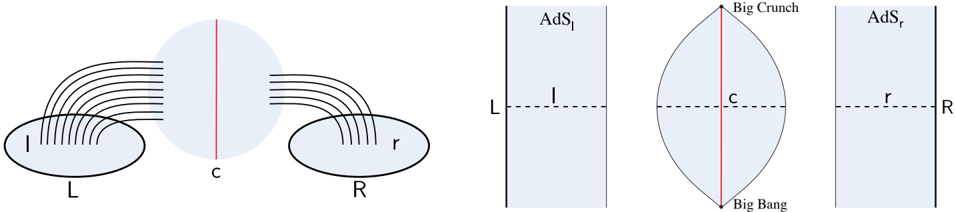
A bstract: Big bang/big crunch closed universes can be realized in AdS/CFT, even though they lack asymptotically AdS boundaries. With enough bulk entanglement, the bulk Hilbert space of a closed universe can be holographically encoded in the CFT. We clarify the relation of this encoding to observer-clone proposals and refute recent arguments about the breakdown of semiclassical physics in such spaces. In the limit of no bulk entanglement, the holographic encoding breaks down. The oft-cited one-dimensional nature of the closed universe Hilbert space represents the limitation of the external (CFT) Hilbert space to access the quantum information in the closed universe, similar to the limitations imposed on observers outside a perfectly isolated quantum lab. We advocate that the CFT nevertheless continues to determine the physical properties of the closed universe in this regime, showing how to interpret this relationship in terms of a final state projection in the closed universe. We provide a dictionary between the final state wavefunction and CFT data. We propose a model of the emergence of an arrow of time in the universe with a given initial or final state projection. Finally, we show that the conventional EFT in the closed universe, without any projection, can be recovered as a maximally ignorant description of the final state. This conventional EFT is encoded in CFT data, and it can be probed by computing coarse-grained observables. We provide an example of one such observable. Taken together, these results amount to a clean bill of health for baby universes born of AdS/CFT. A video abstract is available at https://youtu.be/s_9VqF-N8uQ .
Overview
AI snapshot
Written from the paper’s full text.
TL;DR
The paper revisits the AS2 construction of big-bang/big-crunch closed universes in AdS/CFT and argues that a large closed universe can remain semiclassical even when its Hilbert space appears one-dimensional from the CFT. It refutes a recent SWAP-test argument against semiclassicality, proposes a final-state-projection dictionary between the closed-universe wavefunction and CFT data, and shows conventional closed-universe EFT can be recovered by coarse-graining over final states.
Key findings
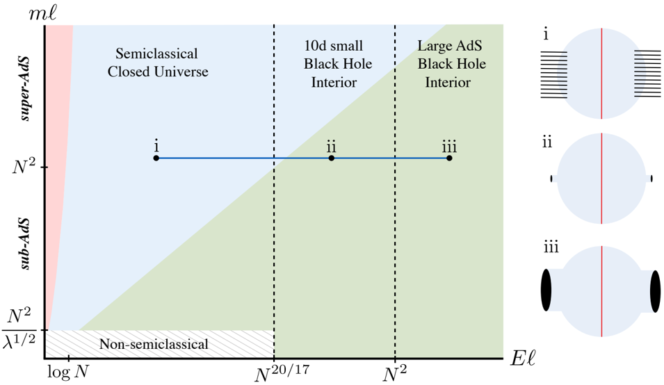
- In the AS2 model, bulk entanglement between the closed universe and AdS regions can be large. In AdS₅×S⁵, the AdS gas entropy is \(S(lr)=(E\ell)^{9/10}\), allowed up to \(E\ell \lesssim O(N^{20/17})\), with \(S(lr)=O(N^{18/17})\) at the transition; the closed-universe entropy is \(S(c)=(m\ell)^2 N^{50/17}\) for \(O(N^2/\lambda^{1/2}) \ll m\ell \ll O(N^2)\), and \(S(c)=m\ell\, N^{16/17}\) for \(O(N^2) \ll m\ell\). The holographic encoding is approximately isometric when \(4S(lr)-3S(c)\gg 1\), effectively isometric when \(S(lr)\gg \log S(c)\), highly non-isometric when \(S(lr)\lesssim \log S(c)\), and breaks down at zero entanglement.
- The EG SWAP test is argued to reduce to the boundary SWAP; for a pure CFT state its expectation value is unity, so it cannot distinguish whether a closed universe is present. The one-dimensional closed-universe Hilbert space is interpreted as the external CFT’s inability to access the closed universe, not as a breakdown of semiclassical physics inside it.
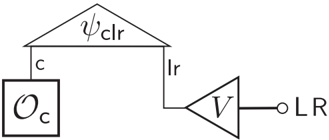
- The paper proposes a final-state projection picture: the CFT determines the final state \(|O_c\rangle\) via the dictionary “final state wavefunction \(\leftrightarrow\) CFT light-light matrix elements of the heavy shell operator \(O\),” \(\Psi_I^O=O_I\). ETH makes this final state quasi-random; averaging over final states gives the maximally mixed \(\rho=\frac{1}{d_c}\mathbb{1}_c\), recovering conventional EFT, while independent replica averaging gives \(\mathrm{rank}(\rho)=d_c\) and correlated averaging gives \(\mathrm{rank}(\rho)=1\).
- CFT experiments can probe closed-universe geometry even at zero entanglement. For example, a two-point function is \(G(\alpha)=e^{-m_A L(\alpha)}\), with \(L(\alpha)=2\ell\log[2\sinh((\alpha+\Delta\tau)/\ell)]\) and \(r_0=\ell\sinh((\alpha+\Delta\tau)/\ell)\); an arrow-of-time toy model yields a Schrödinger-cat-like ground state with eigenvalues \(E_{--}(1\pm|\zeta|+\cdots)\).
Methods
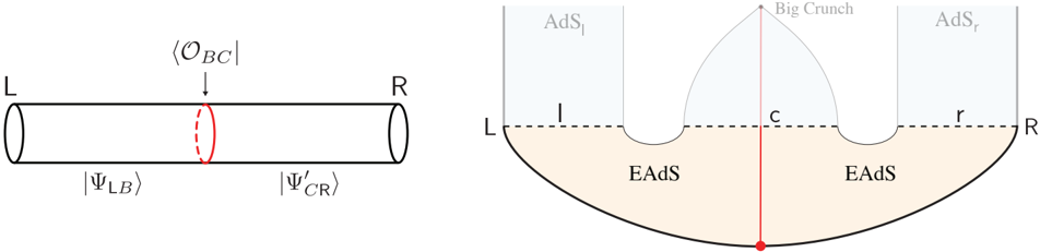
- Reviews and expands the AS2 semiclassical state: two asymptotically AdS regions plus a closed universe supported by a thin dust shell, prepared by Euclidean CFT path integrals/PETS and analyzed via gravitational path-integral saddles and wormholes.
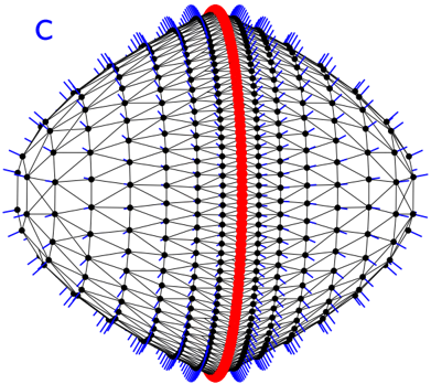
- Uses a random tensor network/MERA model of the holographic map \(W\), Marchenko-Pastur eigenvalue statistics for \(W^\dagger W\), and an ETH ensemble of heavy operators to compute overlaps, variances, Hilbert-space dimensions, and coarse-grained final states.
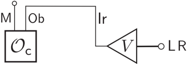
- Proposes CFT protocols with heralded controlled operations and Euclidean evolution to measure matrix elements and reconstruct bulk geometry; includes a canonical quantum gravity argument and numerical exact diagonalization for the arrow-of-time toy model.
Limitations
- Stated: the authors do not claim AdS/CFT will be essential or even useful for describing closed universes in general; the tensor network leaves out details of a full holographic CFT; the Appendix C canonical quantum gravity derivation sweeps many issues under the rug; it is unclear whether local physics from a pure initial/final decoherence functional recovers standard quantum mechanics; complexity limitations are ignored in the proposed CFT experiments; the ETH ansatz for light-light matrix elements lies beyond conventional ETH, with evidence mainly from 2D CFTs and gravity.
- Evident: the results rely on the specific AS2 construction, the heavy-shell limit, Gaussian random tensor/ETH assumptions, and AdS/CFT; no full UV completion or general treatment of arbitrary cosmological singularities is provided.
Model-written summary. Check it against the paper before relying on it.
Integrity signals
Registry
Cites
Statistics
Figures

Verification
Claims the paper makes
189 Own interpretation · 104 No basis given · 45 Not checked yet · 18 Sources not found · 6 Check pending · 6 Own result · 2 No full text of the sources · 1 Supported · 1 Partly supported · 1 Own method · accuracy not yet measured
A check of a cited source is scheduled, or we don’t hold its full text yet; the claim is checked once it runs.
In the paper
“From a counting argument, it then follows from (2.21) that with extremely high probability, the map acts effectively isometrically for all of them as long as the entropy in the closed universe remains sub-exponential in the entropy of the AdS spaces, Splrq “ log Spcq (see [6,68]).”
§ The Baby Universe is Fine and the CFT Knows It: On Holography for Closed Universes > 2.5.2 Effectively isometric regime
What the sources say
- Not checked yetcites [6] S. Antonini, M. Sasieta and B. Swingle, Cosmology from random entanglement, JHEP 11 (2023) 188 [arXiv:2307.14416] [INSPIRE]. source
A check is scheduled.
- Not checked yetcites [68] C. Akers et al., The black hole interior from non-isometric codes and complexity, JHEP 06 (2024) 155 [arXiv:2207.06536] [INSPIRE]. source
A check is scheduled.
boostedconditional- Asserted: passes — The authors put it forward as true.
- Checkable: passes — It can be checked against evidence.
- Load-bearing: passes — The paper’s conclusions depend on it.
- Based: passes — The paper gives a reason why it holds.
- Not checked yet
A check of a cited source is scheduled, or we don’t hold its full text yet; the claim is checked once it runs.
In the paper
“the two-replica wormhole of [6] predicts a statistical variance to the norm of the state”
- Also stated in: § 2.3.1 On the role of operator statistics · plain
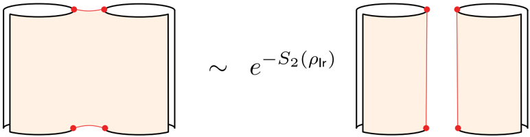
“Z 2 ´Z2 Z 2 “ e ´S2 pρ lr q , (2.9)”
§ The Baby Universe is Fine and the CFT Knows It: On Holography for Closed Universes > 2.3.1 On the role of operator statistics
What the sources say
- Not checked yetcites [6] S. Antonini, M. Sasieta and B. Swingle, Cosmology from random entanglement, JHEP 11 (2023) 188 [arXiv:2307.14416] [INSPIRE]. source
A check is scheduled.
plaindirect- Asserted: passes — The authors put it forward as true.
- Checkable: passes — It can be checked against evidence.
- Load-bearing: passes — The paper’s conclusions depend on it.
- Based: passes — The paper gives a reason why it holds.
- Also stated in: § 2.3.1 On the role of operator statistics · plain
The paper states this without a source or data behind it here, so there is nothing to check it against. The quote shows it is in the paper.
In the paper
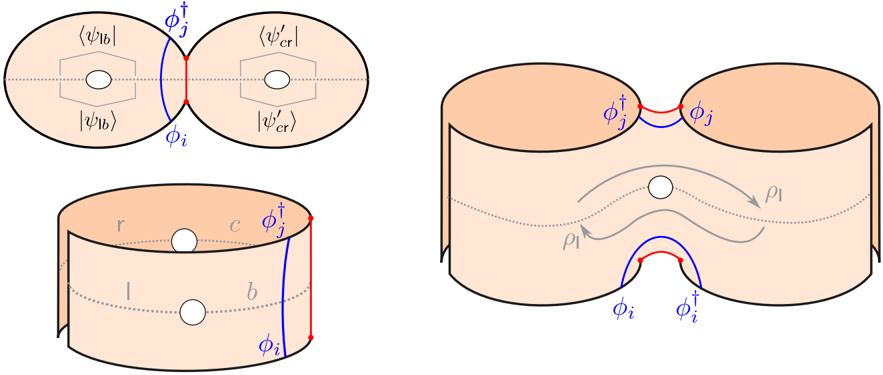
“Its contribution to the overlap is G ij “ δ ij xψ lb |ψ lb y xψ 1 cr |ψ 1 cr y Z 0 e ´mi L i . (3.3)”
§ The Baby Universe is Fine and the CFT Knows It: On Holography for Closed Universes > 3.1 Entanglement and observers in closed universes
plaindirect- Asserted: passes — The authors put it forward as true.
- Checkable: passes — It can be checked against evidence.
- Load-bearing: passes — The paper’s conclusions depend on it.
- Based: passes — The paper gives a reason why it holds.
- The authors state this as an assumption: The heavy shell is not part of the code subspace but is part of a fixed background that holds the universe together.
The paper states this without a source or data behind it here, so there is nothing to check it against. The quote shows it is in the paper.
In the paper
“If these entangled pairs are introduced by inserting particles in the Euclidean preparation, in such a way that they follow geodesics and have well determined positions, we can write the entangled bulk state as |ωy “”
§ The Baby Universe is Fine and the CFT Knows It: On Holography for Closed Universes > 3.1.1 Comments on observers, pointer variables, and all that
plainconditional- Asserted: passes — The authors put it forward as true.
- Checkable: passes — It can be checked against evidence.
- Load-bearing: unclear — It is unclear whether the paper’s conclusions depend on it.
- Based: passes — The paper gives a reason why it holds.
The paper states this without a source or data behind it here, so there is nothing to check it against. The quote shows it is in the paper.
In the paper
“which is determined by the second Rényi entropy of the state of the AdS gases S 2 pρ lr q “ S 2 pρ l q ` S 2 pρ r q, as the state is factorized”
§ The Baby Universe is Fine and the CFT Knows It: On Holography for Closed Universes > 3.1 Entanglement and observers in closed universes
plaindirect- Asserted: passes — The authors put it forward as true.
- Checkable: passes — It can be checked against evidence.
- Load-bearing: passes — The paper’s conclusions depend on it.
- Based: passes — The paper gives a reason why it holds.
- The authors state this as an assumption: The heavy shell is not part of the code subspace but is part of a fixed background that holds the universe together.
None of the sources cited for this claim have been checked yet.
In the paper
“An “external observer α” measures the global SWAP operator of the gases lr (the full LR SWAP), with expectation value 1.”
§ The Baby Universe is Fine and the CFT Knows It: On Holography for Closed Universes > 3.1.1 Comments on observers, pointer variables, and all that
plain- Asserted: passes — The authors put it forward as true.
- Checkable: passes — It can be checked against evidence.
- Load-bearing: unclear — It is unclear whether the paper’s conclusions depend on it.
- Based: passes — The paper gives a reason why it holds.
The paper states this without a source or data behind it here, so there is nothing to check it against. The quote shows it is in the paper.
In the paper
“the rest mass of the shell is essentially mℓ « n∆, where n is the number of particles and ∆ “ 1 is the conformal dimension of the single-particle CFT primary.”
§ The Baby Universe is Fine and the CFT Knows It: On Holography for Closed Universes > 2.4 Parameter space in AdS 5 ˆS5
plaincorrelational- Asserted: passes — The authors put it forward as true.
- Checkable: passes — It can be checked against evidence.
- Load-bearing: unclear — It is unclear whether the paper’s conclusions depend on it.
- Based: passes — The paper gives a reason why it holds.
The paper states this without a source or data behind it here, so there is nothing to check it against. The quote shows it is in the paper.
In the paper
“At low energies, we have AdS spaces which can accommodate gases of particles with an entropy Splrq “ pEℓq 9{10 , (2.10)”
§ The Baby Universe is Fine and the CFT Knows It: On Holography for Closed Universes > 2.4 Parameter space in AdS 5 ˆS5
plaincorrelational- Asserted: passes — The authors put it forward as true.
- Checkable: passes — It can be checked against evidence.
- Load-bearing: passes — The paper’s conclusions depend on it.
- Based: passes — The paper gives a reason why it holds.
The paper states this without a source or data behind it here, so there is nothing to check it against. The quote shows it is in the paper.
In the paper
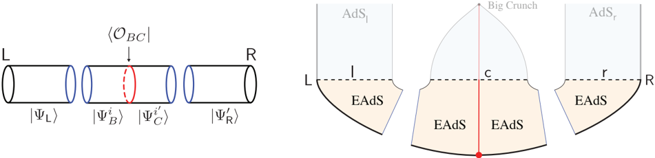
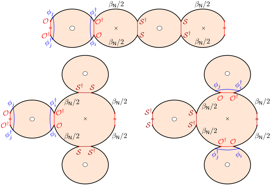
“The presence of the shell does not modify that the dominant Euclidean saddle point is the one in Figure 4 provided that |Ψ LB y and |Ψ 1 CR y correspond to entangled states of two gases of particles in two disconnected AdS factors.”
§ The Baby Universe is Fine and the CFT Knows It: On Holography for Closed Universes > EAdS EAdS
plain- Asserted: passes — The authors put it forward as true.
- Checkable: passes — It can be checked against evidence.
- Load-bearing: passes — The paper’s conclusions depend on it.
- Based: passes — The paper gives a reason why it holds.
None of the sources cited for this claim have been checked yet.
In the paper
“For the random tensor model of Figure 7, the overlap between two states |ψ M y , |ϕ M y is preserved on average, up to exponentially small errors in the entropy,”
§ The Baby Universe is Fine and the CFT Knows It: On Holography for Closed Universes > 2.5.2 Effectively isometric regime
plain- Asserted: passes — The authors put it forward as true.
- Checkable: passes — It can be checked against evidence.
- Load-bearing: passes — The paper’s conclusions depend on it.
- Based: passes — The paper gives a reason why it holds.
In the paper
“The expectation value of the partial SWAP operator for the external gas (the R CFT SWAP) is the maximum between e ´S2 prq and e ´S2 plq , just like in [58].”
§ The Baby Universe is Fine and the CFT Knows It: On Holography for Closed Universes > 3.1.1 Comments on observers, pointer variables, and all that
What the sources say
- Not matchedcites [58] N. Engelhardt, E. Gesteau and D. Harlow, Observer complementarity for black holes and holography, arXiv:2507.06046 [INSPIRE].
Couldn’t be matched to a paper in Crossref, so it can’t be checked.
plaincorrelational- Asserted: passes — The authors put it forward as true.
- Checkable: passes — It can be checked against evidence.
- Load-bearing: unclear — It is unclear whether the paper’s conclusions depend on it.
- Based: passes — The paper gives a reason why it holds.
- Not matched
The paper states this without a source or data behind it here, so there is nothing to check it against. The quote shows it is in the paper.
In the paper
“In this random tensor model, W : W corresponds to a Wishart random matrix.”
§ The Baby Universe is Fine and the CFT Knows It: On Holography for Closed Universes > 2.5.1 Approximately isometric regime
plaincorrelational- Asserted: passes — The authors put it forward as true.
- Checkable: passes — It can be checked against evidence.
- Load-bearing: passes — The paper’s conclusions depend on it.
- Based: passes — The paper gives a reason why it holds.
The paper states this without a source or data behind it here, so there is nothing to check it against. The quote shows it is in the paper.
In the paper
“Therefore, the Euclidean manifold effectively factorizes into two Euclidean manifolds.”
§ The Baby Universe is Fine and the CFT Knows It: On Holography for Closed Universes > EAdS EAdS
plaindirect- Asserted: passes — The authors put it forward as true.
- Checkable: passes — It can be checked against evidence.
- Load-bearing: passes — The paper’s conclusions depend on it.
- Based: passes — The paper gives a reason why it holds.
The paper states this without a source or data behind it here, so there is nothing to check it against. The quote shows it is in the paper.
In the paper
“On average over the Gaussian random state |O c y, the map W is isometric, W : W “ 1 M for any ratio of the bond dimensions.”
§ The Baby Universe is Fine and the CFT Knows It: On Holography for Closed Universes > 2.5.1 Approximately isometric regime
plain- Asserted: passes — The authors put it forward as true.
- Checkable: passes — It can be checked against evidence.
- Load-bearing: passes — The paper’s conclusions depend on it.
- Based: passes — The paper gives a reason why it holds.
The paper states this without a source or data behind it here, so there is nothing to check it against. The quote shows it is in the paper.
In the paper
“The variance of the dimension, computed gravitationally, vanishes, up to possible off-shell contributions.”
§ The Baby Universe is Fine and the CFT Knows It: On Holography for Closed Universes > 3.1 Entanglement and observers in closed universes
hedged- Asserted: passes — The authors put it forward as true.
- Checkable: passes — It can be checked against evidence.
- Load-bearing: passes — The paper’s conclusions depend on it.
- Based: passes — The paper gives a reason why it holds.
- The authors state this as an assumption: The heavy shell is not part of the code subspace but is part of a fixed background that holds the universe together.
The paper states this without a source or data behind it here, so there is nothing to check it against. The quote shows it is in the paper.
In the paper
“In our setup, this is simply bulk entanglement entropy between the closed universe and AdS r .”
§ The Baby Universe is Fine and the CFT Knows It: On Holography for Closed Universes > 1.1 FAQ
plaincorrelational- Asserted: passes — The authors put it forward as true.
- Checkable: passes — It can be checked against evidence.
- Load-bearing: unclear — It is unclear whether the paper’s conclusions depend on it.
- Based: passes — The paper gives a reason why it holds.
The paper states this without a source or data behind it here, so there is nothing to check it against. The quote shows it is in the paper.
In the paper
“The semiclassical state is prepared by a Euclidean gravitational solution with boundary conditions fixed by the corresponding CFT path integral, as shown in Figure 4.”
§ The Baby Universe is Fine and the CFT Knows It: On Holography for Closed Universes > EAdS EAdS
boosteddirect- Asserted: passes — The authors put it forward as true.
- Checkable: passes — It can be checked against evidence.
- Load-bearing: passes — The paper’s conclusions depend on it.
- Based: passes — The paper gives a reason why it holds.
In the paper
“The results for a closed universe presented there are reproduced in our setup using the language of observers as described in this section.”
§ The Baby Universe is Fine and the CFT Knows It: On Holography for Closed Universes > 3.1.1 Comments on observers, pointer variables, and all that
What the sources say
- Not matchedcites [58] N. Engelhardt, E. Gesteau and D. Harlow, Observer complementarity for black holes and holography, arXiv:2507.06046 [INSPIRE].
Couldn’t be matched to a paper in Crossref, so it can’t be checked.
plaincorrelational- Asserted: passes — The authors put it forward as true.
- Checkable: passes — It can be checked against evidence.
- Load-bearing: unclear — It is unclear whether the paper’s conclusions depend on it.
- Based: passes — The paper gives a reason why it holds.
- Not matched
The paper states this without a source or data behind it here, so there is nothing to check it against. The quote shows it is in the paper.
In the paper
“The mass density of the shell remains parametrically smaller than the Planck density.”
§ The Baby Universe is Fine and the CFT Knows It: On Holography for Closed Universes > Big Crunch AdS
plain- Asserted: passes — The authors put it forward as true.
- Checkable: passes — It can be checked against evidence.
- Load-bearing: unclear — It is unclear whether the paper’s conclusions depend on it.
- Based: unclear — It is unclear why the paper says it holds.
A check of a cited source is scheduled, or we don’t hold its full text yet; the claim is checked once it runs.
In the paper
“In the large bond dimension limit, the eigenvalues λ of W : W are distributed according to the Marchenko-Pastur distribution [96]”
- Also stated in: § 2.5.1 Approximately isometric regime · plain
“λ ˘“ p1 ˘?rq 2 . (2.15)”
§ The Baby Universe is Fine and the CFT Knows It: On Holography for Closed Universes > 2.5.1 Approximately isometric regime
What the sources say
- Not checked yetcites [96] L.A. Pastur and V.A. Marčenko, Distribution of Eigenvalues for Some Sets of Random Matrices, Math. USSR Sb. 1 (1967) 457 [INSPIRE]. source
A check is scheduled.
plaincorrelational- Asserted: passes — The authors put it forward as true.
- Checkable: passes — It can be checked against evidence.
- Load-bearing: passes — The paper’s conclusions depend on it.
- Based: passes — The paper gives a reason why it holds.
- Also stated in: § 2.5.1 Approximately isometric regime · plain
The paper states this without a source or data behind it here, so there is nothing to check it against. The quote shows it is in the paper.
In the paper
“This expression agrees with the variance-to-norm squared ratio of Z over an ensemble of microscopic thin shell operators.”
§ The Baby Universe is Fine and the CFT Knows It: On Holography for Closed Universes > 2.3.1 On the role of operator statistics
plaincorrelational- Asserted: passes — The authors put it forward as true.
- Checkable: passes — It can be checked against evidence.
- Load-bearing: passes — The paper’s conclusions depend on it.
- Based: passes — The paper gives a reason why it holds.
The paper states this without a source or data behind it here, so there is nothing to check it against. The quote shows it is in the paper.
In the paper
“If the mass of the shell is sufficiently large, its trajectory always remains in the asymptotic AdS region in the Euclidean diagram of Figure 4, independent of other matter fields.”
§ The Baby Universe is Fine and the CFT Knows It: On Holography for Closed Universes > EAdS EAdS
plaindirect- Asserted: passes — The authors put it forward as true.
- Checkable: passes — It can be checked against evidence.
- Load-bearing: passes — The paper’s conclusions depend on it.
- Based: unclear — It is unclear why the paper says it holds.
A check of a cited source is scheduled, or we don’t hold its full text yet; the claim is checked once it runs.
In the paper
“From (3.5) and the higher moments, a conventional resolvent calculation outlined in [6] yields that the states |Ψ i y span the microcanonical Hilbert space dimension of the clone, dimpH Ob 1 q “ rankpG ij q “ e Splrq . (3.6)”
§ The Baby Universe is Fine and the CFT Knows It: On Holography for Closed Universes > 3.1 Entanglement and observers in closed universes
What the sources say
- Not checked yetcites [6] S. Antonini, M. Sasieta and B. Swingle, Cosmology from random entanglement, JHEP 11 (2023) 188 [arXiv:2307.14416] [INSPIRE]. source
A check is scheduled.
plaindirect- Asserted: passes — The authors put it forward as true.
- Checkable: passes — It can be checked against evidence.
- Load-bearing: passes — The paper’s conclusions depend on it.
- Based: passes — The paper gives a reason why it holds.
- The authors state this as an assumption: The heavy shell is not part of the code subspace but is part of a fixed background that holds the universe together.
- Not checked yet
The paper states this without a source or data behind it here, so there is nothing to check it against. The quote shows it is in the paper.
In the paper
“One could then apply this version of the causal wedge SWAP to an”
§ The Baby Universe is Fine and the CFT Knows It: On Holography for Closed Universes > 3.2.3 How to not swap the closed universes
hedgeddirect- Asserted: passes — The authors put it forward as true.
- Checkable: passes — It can be checked against evidence.
- Load-bearing: unclear — It is unclear whether the paper’s conclusions depend on it.
- Based: passes — The paper gives a reason why it holds.
The paper states this without a source or data behind it here, so there is nothing to check it against. The quote shows it is in the paper.
In the paper
“Regardless of whether we consider a bulk description with or without a closed universe (Descriptions 1 and 2 in AR, respectively), the expectation value of the SWAP operator will always give unity.”
§ The Baby Universe is Fine and the CFT Knows It: On Holography for Closed Universes > 3.2.2 Addressing the EG argument
plain- Asserted: passes — The authors put it forward as true.
- Checkable: passes — It can be checked against evidence.
- Load-bearing: passes — The paper’s conclusions depend on it.
- Based: passes — The paper gives a reason why it holds.
The paper states this without a source or data behind it here, so there is nothing to check it against. The quote shows it is in the paper.
In the paper
“In this case, there is an effectively isometric encoding (strictly non-isometric) of the closed universe in the CFT.”
§ The Baby Universe is Fine and the CFT Knows It: On Holography for Closed Universes > 5.3 Reconstructing the closed universe from CFT data
plainconditional- Asserted: passes — The authors put it forward as true.
- Checkable: passes — It can be checked against evidence.
- Load-bearing: passes — The paper’s conclusions depend on it.
- Based: passes — The paper gives a reason why it holds.
The paper states this without a source or data behind it here, so there is nothing to check it against. The quote shows it is in the paper.
In the paper
“In the limit of low temperatures, β L,R Ñ 8, the state reduces to”
§ The Baby Universe is Fine and the CFT Knows It: On Holography for Closed Universes > 5.3 Reconstructing the closed universe from CFT data
plaindirect- Asserted: passes — The authors put it forward as true.
- Checkable: passes — It can be checked against evidence.
- Load-bearing: passes — The paper’s conclusions depend on it.
- Based: passes — The paper gives a reason why it holds.
- The authors state this as an assumption: The erratic parts of the heavy operator's matrix elements behave as i.i.d. random complex Gaussian variables.
The paper states this without a source or data behind it here, so there is nothing to check it against. The quote shows it is in the paper.
In the paper
“In fact, α is related to the radial location r 0 of the bulk particle in the closed universe at the reflection symmetric slice by”
§ The Baby Universe is Fine and the CFT Knows It: On Holography for Closed Universes > 5.3 Reconstructing the closed universe from CFT data
plaincorrelational- Asserted: passes — The authors put it forward as true.
- Checkable: passes — It can be checked against evidence.
- Load-bearing: passes — The paper’s conclusions depend on it.
- Based: passes — The paper gives a reason why it holds.
- The authors state this as an assumption: The erratic parts of the heavy operator's matrix elements behave as i.i.d. random complex Gaussian variables.
The paper states this without a source or data behind it here, so there is nothing to check it against. The quote shows it is in the paper.
In the paper
“The length is given by”
§ The Baby Universe is Fine and the CFT Knows It: On Holography for Closed Universes > 5.3 Reconstructing the closed universe from CFT data
plaindirect- Asserted: passes — The authors put it forward as true.
- Checkable: passes — It can be checked against evidence.
- Load-bearing: passes — The paper’s conclusions depend on it.
- Based: passes — The paper gives a reason why it holds.
- The authors state this as an assumption: The erratic parts of the heavy operator's matrix elements behave as i.i.d. random complex Gaussian variables.
The paper states this without a source or data behind it here, so there is nothing to check it against. The quote shows it is in the paper.
In the paper
“These two states are mapped into each other under time-reversal,”
§ The Baby Universe is Fine and the CFT Knows It: On Holography for Closed Universes > 4.4 Arrow of time
plaindirect- Asserted: passes — The authors put it forward as true.
- Checkable: passes — It can be checked against evidence.
- Load-bearing: unclear — It is unclear whether the paper’s conclusions depend on it.
- Based: passes — The paper gives a reason why it holds.
- The authors state this as an assumption: The system Hamiltonian H is a random GOE matrix.
- The authors state this as an assumption: The CR action is trivial.
- The authors state this as an assumption: The system and clock are non-interacting.
A result the paper reports from its own data — it cites no other source for it, so there is none to check. The quote shows it is in the paper.
In the paper
“We exhibit a toy model in which the ground state of a Wheeler-DeWitt-like Hamiltonian spontaneously breaks time-reversal symmetry by taking the form of a Schrodinger's cat like state.”
§ The Baby Universe is Fine and the CFT Knows It: On Holography for Closed Universes > 4.4 Arrow of time
boosteddirect- Asserted: passes — The authors put it forward as true.
- Checkable: passes — It can be checked against evidence.
- Load-bearing: passes — The paper’s conclusions depend on it.
- Based: passes — The paper gives a reason why it holds.
- The authors state this as an assumption: The system Hamiltonian H is a random GOE matrix.
- The authors state this as an assumption: The CR action is trivial.
- The authors state this as an assumption: The system and clock are non-interacting.
A result the paper reports from its own data — it cites no other source for it, so there is none to check. The quote shows it is in the paper.
In the paper
“However, |Ψ ´y and |Ψ `y are not orthogonal states, so we first construct an orthonormal basis to find the eigenvalues of H SC in the subspace.”
§ The Baby Universe is Fine and the CFT Knows It: On Holography for Closed Universes > 4.4 Arrow of time
plain- Asserted: passes — The authors put it forward as true.
- Checkable: passes — It can be checked against evidence.
- Load-bearing: passes — The paper’s conclusions depend on it.
- Based: passes — The paper gives a reason why it holds.
- The authors state this as an assumption: The system Hamiltonian H is a random GOE matrix.
- The authors state this as an assumption: The CR action is trivial.
- The authors state this as an assumption: The system and clock are non-interacting.
The paper states this without a source or data behind it here, so there is nothing to check it against. The quote shows it is in the paper.
In the paper
“Crucially, however, the cross matrix element is small for a generic O,”
§ The Baby Universe is Fine and the CFT Knows It: On Holography for Closed Universes > 4.4 Arrow of time
plain- Asserted: passes — The authors put it forward as true.
- Checkable: passes — It can be checked against evidence.
- Load-bearing: passes — The paper’s conclusions depend on it.
- Based: passes — The paper gives a reason why it holds.
- The authors state this as an assumption: The system Hamiltonian H is a random GOE matrix.
- The authors state this as an assumption: The CR action is trivial.
- The authors state this as an assumption: The system and clock are non-interacting.
The paper states this without a source or data behind it here, so there is nothing to check it against. The quote shows it is in the paper.
In the paper
“It is possible that, for special choices of |ψ 0 y and H, both H init and H final can be satisfied, but this is not generic.”
§ The Baby Universe is Fine and the CFT Knows It: On Holography for Closed Universes > 4.4 Arrow of time
hedged- Asserted: passes — The authors put it forward as true.
- Checkable: passes — It can be checked against evidence.
- Load-bearing: passes — The paper’s conclusions depend on it.
- Based: passes — The paper gives a reason why it holds.
- The authors state this as an assumption: The system Hamiltonian H is a random GOE matrix.
- The authors state this as an assumption: The CR action is trivial.
- The authors state this as an assumption: The system and clock are non-interacting.
The paper states this without a source or data behind it here, so there is nothing to check it against. The quote shows it is in the paper.
In the paper
“The coarse-grained final state is then, using the explicit form of the Gaussian measure”
§ The Baby Universe is Fine and the CFT Knows It: On Holography for Closed Universes > 5.2.2 Connection to α-states in a many-universe Hilbert space
plaincorrelational- Asserted: passes — The authors put it forward as true.
- Checkable: passes — It can be checked against evidence.
- Load-bearing: passes — The paper’s conclusions depend on it.
- Based: passes — The paper gives a reason why it holds.
- The authors state this as an assumption: The erratic parts of the heavy operator's matrix elements behave as i.i.d. random complex Gaussian variables.
The paper states this without a source or data behind it here, so there is nothing to check it against. The quote shows it is in the paper.
In the paper
“Thus, we find that the average state is maximally mixed”
§ The Baby Universe is Fine and the CFT Knows It: On Holography for Closed Universes > 5.2 Statistical average over final states
plain- Asserted: passes — The authors put it forward as true.
- Checkable: passes — It can be checked against evidence.
- Load-bearing: passes — The paper’s conclusions depend on it.
- Based: passes — The paper gives a reason why it holds.
- The authors state this as an assumption: The erratic parts of the heavy operator's matrix elements behave as i.i.d. random complex Gaussian variables.
A result the paper reports from its own data — it cites no other source for it, so there is none to check. The quote shows it is in the paper.
In the paper
“In Section 2.4, we discussed in detail the specific case of Type IIB string theory dual to N”
§ The Baby Universe is Fine and the CFT Knows It: On Holography for Closed Universes > 5.3 Reconstructing the closed universe from CFT data
plaincorrelational- Asserted: passes — The authors put it forward as true.
- Checkable: passes — It can be checked against evidence.
- Load-bearing: passes — The paper’s conclusions depend on it.
- Based: passes — The paper gives a reason why it holds.
The paper states this without a source or data behind it here, so there is nothing to check it against. The quote shows it is in the paper.
In the paper
“In general, for a pd `1q-dimensional AdS, its entanglement entropy to the closed universe is upper bounded by OpN 2d{p2d´1q q, corresponding to the entropy of the most entropic stable gas in AdS.”
§ The Baby Universe is Fine and the CFT Knows It: On Holography for Closed Universes > 5.3 Reconstructing the closed universe from CFT data
plaincorrelational- Asserted: passes — The authors put it forward as true.
- Checkable: passes — It can be checked against evidence.
- Load-bearing: passes — The paper’s conclusions depend on it.
- Based: unclear — It is unclear why the paper says it holds.
The paper states this without a source or data behind it here, so there is nothing to check it against. The quote shows it is in the paper.
In the paper
“The ground state thus amounts to a Schrodinger's cat-like state for time-reversal symmetry.”
§ The Baby Universe is Fine and the CFT Knows It: On Holography for Closed Universes > 4.4 Arrow of time
plaincorrelational- Asserted: passes — The authors put it forward as true.
- Checkable: passes — It can be checked against evidence.
- Load-bearing: unclear — It is unclear whether the paper’s conclusions depend on it.
- Based: passes — The paper gives a reason why it holds.
- The authors state this as an assumption: The system Hamiltonian H is a random GOE matrix.
- The authors state this as an assumption: The CR action is trivial.
- The authors state this as an assumption: The system and clock are non-interacting.
The paper states this without a source or data behind it here, so there is nothing to check it against. The quote shows it is in the paper.
In the paper
“The statistical average over final states is given by”
§ The Baby Universe is Fine and the CFT Knows It: On Holography for Closed Universes > 5.2 Statistical average over final states
plain- Asserted: passes — The authors put it forward as true.
- Checkable: passes — It can be checked against evidence.
- Load-bearing: passes — The paper’s conclusions depend on it.
- Based: passes — The paper gives a reason why it holds.
- The authors state this as an assumption: The erratic parts of the heavy operator's matrix elements behave as i.i.d. random complex Gaussian variables.
The paper states this without a source or data behind it here, so there is nothing to check it against. The quote shows it is in the paper.
In the paper
“The matrix element xgs|O piq |gsy, computed in gravity, vanishes.”
§ The Baby Universe is Fine and the CFT Knows It: On Holography for Closed Universes > 5.1 ETH ensemble
plain- Asserted: passes — The authors put it forward as true.
- Checkable: passes — It can be checked against evidence.
- Load-bearing: passes — The paper’s conclusions depend on it.
- Based: passes — The paper gives a reason why it holds.
- The authors state this as an assumption: The erratic parts of the heavy operator's matrix elements behave as i.i.d. random complex Gaussian variables.
The paper states this without a source or data behind it here, so there is nothing to check it against. The quote shows it is in the paper.
In the paper
“It follows from (4.6) that the final state of the closed universe is quasi-random.”
§ The Baby Universe is Fine and the CFT Knows It: On Holography for Closed Universes > 4.3.2 Singularities and quantum chaos
plaindirect- Asserted: passes — The authors put it forward as true.
- Checkable: passes — It can be checked against evidence.
- Load-bearing: passes — The paper’s conclusions depend on it.
- Based: passes — The paper gives a reason why it holds.
- The authors state this as an assumption: The erratic parts of the heavy operator's matrix elements behave as i.i.d. random complex Gaussian variables.
The paper states this without a source or data behind it here, so there is nothing to check it against. The quote shows it is in the paper.
In the paper
“Finally, we explicitly showed an example of a CFT observable, together with sufficient statistics, which can probe [QFT] in the closed universe even in the absence of any entanglement in the [QFT] description.”
§ The Baby Universe is Fine and the CFT Knows It: On Holography for Closed Universes > 5.3 Reconstructing the closed universe from CFT data
boosteddirect- Asserted: passes — The authors put it forward as true.
- Checkable: passes — It can be checked against evidence.
- Load-bearing: passes — The paper’s conclusions depend on it.
- Based: passes — The paper gives a reason why it holds.
The paper states this without a source or data behind it here, so there is nothing to check it against. The quote shows it is in the paper.
In the paper
“This conclusion is unchanged if the measurements are performed within sufficiently small subsystems and one starts from the global decoherence functional.”
§ The Baby Universe is Fine and the CFT Knows It: On Holography for Closed Universes > 5.3 Reconstructing the closed universe from CFT data
plain- Asserted: passes — The authors put it forward as true.
- Checkable: passes — It can be checked against evidence.
- Load-bearing: unclear — It is unclear whether the paper’s conclusions depend on it.
- Based: passes — The paper gives a reason why it holds.
The paper states this without a source or data behind it here, so there is nothing to check it against. The quote shows it is in the paper.
In the paper
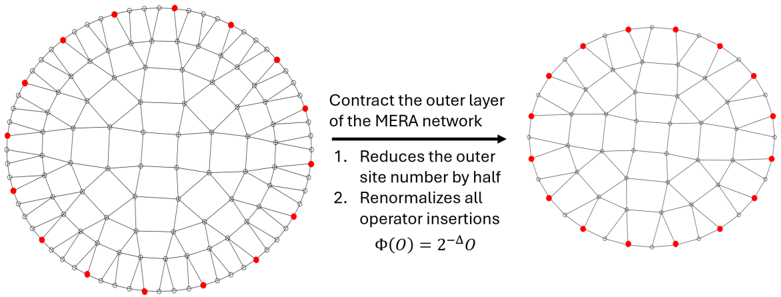
“This contraction can be safely continued until the operator insertions are adjacent to each other at the lattice scale.”
§ The Baby Universe is Fine and the CFT Knows It: On Holography for Closed Universes > 5.3 Reconstructing the closed universe from CFT data
plain- Asserted: passes — The authors put it forward as true.
- Checkable: passes — It can be checked against evidence.
- Load-bearing: passes — The paper’s conclusions depend on it.
- Based: passes — The paper gives a reason why it holds.
The paper states this without a source or data behind it here, so there is nothing to check it against. The quote shows it is in the paper.
In the paper
“Now, when both g init and g final are zero, then any state of the form (4.14) for any |ψy is a zero energy state of H SC .”
§ The Baby Universe is Fine and the CFT Knows It: On Holography for Closed Universes > 4.4 Arrow of time
plain- Asserted: passes — The authors put it forward as true.
- Checkable: passes — It can be checked against evidence.
- Load-bearing: passes — The paper’s conclusions depend on it.
- Based: passes — The paper gives a reason why it holds.
- The authors state this as an assumption: The system Hamiltonian H is a random GOE matrix.
- The authors state this as an assumption: The CR action is trivial.
- The authors state this as an assumption: The system and clock are non-interacting.
The paper states this without a source or data behind it here, so there is nothing to check it against. The quote shows it is in the paper.
In the paper
“Within the ETH ensemble of operators, the matrix element xgs|O piq |gsy is a random variable with zero mean and non-zero variance.”
§ The Baby Universe is Fine and the CFT Knows It: On Holography for Closed Universes > 5.3 Reconstructing the closed universe from CFT data
plain- Asserted: passes — The authors put it forward as true.
- Checkable: passes — It can be checked against evidence.
- Load-bearing: passes — The paper’s conclusions depend on it.
- Based: passes — The paper gives a reason why it holds.
- The authors state this as an assumption: The erratic parts of the heavy operator's matrix elements behave as i.i.d. random complex Gaussian variables.
The paper states this without a source or data behind it here, so there is nothing to check it against. The quote shows it is in the paper.
In the paper
“Taking the normalization 1{ ?Z i into account, the state (5.13) is the vacuum up to a phase”
§ The Baby Universe is Fine and the CFT Knows It: On Holography for Closed Universes > 5.3 Reconstructing the closed universe from CFT data
plaincorrelational- Asserted: passes — The authors put it forward as true.
- Checkable: passes — It can be checked against evidence.
- Load-bearing: passes — The paper’s conclusions depend on it.
- Based: passes — The paper gives a reason why it holds.
- The authors state this as an assumption: The erratic parts of the heavy operator's matrix elements behave as i.i.d. random complex Gaussian variables.
The paper states this without a source or data behind it here, so there is nothing to check it against. The quote shows it is in the paper.
In the paper
“Because the on-shell gravitational action of the saddle is the same in the numerator and denominator, the two-point function reduces to”
§ The Baby Universe is Fine and the CFT Knows It: On Holography for Closed Universes > 5.3 Reconstructing the closed universe from CFT data
plaindirect- Asserted: passes — The authors put it forward as true.
- Checkable: passes — It can be checked against evidence.
- Load-bearing: passes — The paper’s conclusions depend on it.
- Based: passes — The paper gives a reason why it holds.
- The authors state this as an assumption: The erratic parts of the heavy operator's matrix elements behave as i.i.d. random complex Gaussian variables.
The paper states this without a source or data behind it here, so there is nothing to check it against. The quote shows it is in the paper.
In the paper
“As an example, for two replica quantities, the average state is”
§ The Baby Universe is Fine and the CFT Knows It: On Holography for Closed Universes > 5.2.1 Replicas and dimensions
plaincorrelational- Asserted: passes — The authors put it forward as true.
- Checkable: passes — It can be checked against evidence.
- Load-bearing: unclear — It is unclear whether the paper’s conclusions depend on it.
- Based: passes — The paper gives a reason why it holds.
- The authors state this as an assumption: The erratic parts of the heavy operator's matrix elements behave as i.i.d. random complex Gaussian variables.
The paper states this without a source or data behind it here, so there is nothing to check it against. The quote shows it is in the paper.
In the paper
“From the CFT perspective, the answer is clear: the state is pure and the SWAP test will give unity.”
- Also stated in: § 3.2.5 Closing comments · plain
“the result of such a SWAP test on the CFT state is unit purity.”
§ The Baby Universe is Fine and the CFT Knows It: On Holography for Closed Universes > 3.2.2 Addressing the EG argument
boosteddirect- Asserted: passes — The authors put it forward as true.
- Checkable: passes — It can be checked against evidence.
- Load-bearing: passes — The paper’s conclusions depend on it.
- Based: passes — The paper gives a reason why it holds.
- Also stated in: § 3.2.5 Closing comments · plain
The paper states this without a source or data behind it here, so there is nothing to check it against. The quote shows it is in the paper.
In the paper
“Using this notation, if we compute expectation values in an α-state instead of in the oscillator vacuum,”
§ The Baby Universe is Fine and the CFT Knows It: On Holography for Closed Universes > 5.2.2 Connection to α-states in a many-universe Hilbert space
hedgeddirect- Asserted: passes — The authors put it forward as true.
- Checkable: passes — It can be checked against evidence.
- Load-bearing: passes — The paper’s conclusions depend on it.
- Based: passes — The paper gives a reason why it holds.
- The authors state this as an assumption: The erratic parts of the heavy operator's matrix elements behave as i.i.d. random complex Gaussian variables.
The paper states this without a source or data behind it here, so there is nothing to check it against. The quote shows it is in the paper.
In the paper
“Second, the bulk states generically share entanglement between the AdS regions and the closed universe.”
§ The Baby Universe is Fine and the CFT Knows It: On Holography for Closed Universes > 5.3 Reconstructing the closed universe from CFT data
plaincorrelational- Asserted: passes — The authors put it forward as true.
- Checkable: passes — It can be checked against evidence.
- Load-bearing: passes — The paper’s conclusions depend on it.
- Based: passes — The paper gives a reason why it holds.
The paper states this without a source or data behind it here, so there is nothing to check it against. The quote shows it is in the paper.
In the paper
“The expectation values of two different operators O piq , O pjq are uncorrelated in this approximation,”
§ The Baby Universe is Fine and the CFT Knows It: On Holography for Closed Universes > 5.3 Reconstructing the closed universe from CFT data
hedged- Asserted: passes — The authors put it forward as true.
- Checkable: passes — It can be checked against evidence.
- Load-bearing: passes — The paper’s conclusions depend on it.
- Based: passes — The paper gives a reason why it holds.
- The authors state this as an assumption: The erratic parts of the heavy operator's matrix elements behave as i.i.d. random complex Gaussian variables.
A check of a cited source is scheduled, or we don’t hold its full text yet; the claim is checked once it runs.
In the paper
“To recall the basic elements of the setup, there exist entangled states between two copies of a holographic CFT whose dual spacetime is formed by three disconnected pieces: two AdS regions and a crunching closed universe supported by a thin shell of dust.”
§ The Baby Universe is Fine and the CFT Knows It: On Holography for Closed Universes > 5.3 Reconstructing the closed universe from CFT data
What the sources say
- Not checked yetcites [6] S. Antonini, M. Sasieta and B. Swingle, Cosmology from random entanglement, JHEP 11 (2023) 188 [arXiv:2307.14416] [INSPIRE]. source
A check is scheduled.
plaincorrelational- Asserted: passes — The authors put it forward as true.
- Checkable: passes — It can be checked against evidence.
- Load-bearing: passes — The paper’s conclusions depend on it.
- Based: passes — The paper gives a reason why it holds.
- Not checked yet
The paper states this without a source or data behind it here, so there is nothing to check it against. The quote shows it is in the paper.
In the paper
“We will find a Page curve-like behavior that allows us to estimate the size of the Hilbert space we are entangling the external system with.”
§ The Baby Universe is Fine and the CFT Knows It: On Holography for Closed Universes > Additional information
plaindirect- Asserted: passes — The authors put it forward as true.
- Checkable: passes — It can be checked against evidence.
- Load-bearing: passes — The paper’s conclusions depend on it.
- Based: passes — The paper gives a reason why it holds.
- The authors state this as an assumption: At least one of S(ρ_l) or S(ρ_r) is large.
The paper states this without a source or data behind it here, so there is nothing to check it against. The quote shows it is in the paper.
In the paper
“The square of the overlaps has now, in addition to the disconnected contribution, three other saddle point geometries depending on how the thin shells are contracted.”
§ The Baby Universe is Fine and the CFT Knows It: On Holography for Closed Universes > Additional information
plaincorrelational- Asserted: passes — The authors put it forward as true.
- Checkable: passes — It can be checked against evidence.
- Load-bearing: unclear — It is unclear whether the paper’s conclusions depend on it.
- Based: passes — The paper gives a reason why it holds.
The paper states this without a source or data behind it here, so there is nothing to check it against. The quote shows it is in the paper.
In the paper
“If we try to increase K without bound, the second Rényi of the auxiliary system is limited by the minimum between S 2 pρ l q `S2 pρ r q and S 2 pρ l q `S2 pβ N q.”
§ The Baby Universe is Fine and the CFT Knows It: On Holography for Closed Universes > Additional information
plaindirect- Asserted: passes — The authors put it forward as true.
- Checkable: passes — It can be checked against evidence.
- Load-bearing: passes — The paper’s conclusions depend on it.
- Based: passes — The paper gives a reason why it holds.
- The authors state this as an assumption: At least one of S(ρ_l) or S(ρ_r) is large.
- Rests on an assumption: The fluctuations of the norm of the CFT states are suppressed, allowing normalization with the average.
The paper states this without a source or data behind it here, so there is nothing to check it against. The quote shows it is in the paper.
In the paper
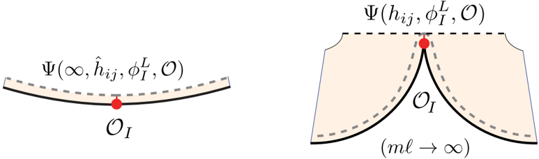
“In this limit, the Euclidean action I E has local divergences that can be renormalized with suitable counterterms using a conventional scheme of holographic renormalization.”
§ The Baby Universe is Fine and the CFT Knows It: On Holography for Closed Universes > C Gravitational argument for the final state wavefunction
plaindirect- Asserted: passes — The authors put it forward as true.
- Checkable: passes — It can be checked against evidence.
- Load-bearing: passes — The paper’s conclusions depend on it.
- Based: unclear — It is unclear why the paper says it holds.
The paper states this without a source or data behind it here, so there is nothing to check it against. The quote shows it is in the paper.
In the paper
“Using multiple thin shells, we can construct closed universes that have geometric features not present in the ones discussed in the main text.”
§ The Baby Universe is Fine and the CFT Knows It: On Holography for Closed Universes > B Closed universe with a geometric bottleneck
plaindirect- Asserted: passes — The authors put it forward as true.
- Checkable: passes — It can be checked against evidence.
- Load-bearing: unclear — It is unclear whether the paper’s conclusions depend on it.
- Based: passes — The paper gives a reason why it holds.
The paper states this without a source or data behind it here, so there is nothing to check it against. The quote shows it is in the paper.
In the paper
“The renormalized final state wavefunction is then equal to the CFT path integral lim aÑ8 Ψpa, ĥij , ϕ I q ren”
§ The Baby Universe is Fine and the CFT Knows It: On Holography for Closed Universes > C Gravitational argument for the final state wavefunction
plaincorrelational- Asserted: passes — The authors put it forward as true.
- Checkable: passes — It can be checked against evidence.
- Load-bearing: passes — The paper’s conclusions depend on it.
- Based: passes — The paper gives a reason why it holds.
The paper states this without a source or data behind it here, so there is nothing to check it against. The quote shows it is in the paper.
In the paper
“The typical size of the variance of the inner products is thus controlled by the competition between the various terms,”
§ The Baby Universe is Fine and the CFT Knows It: On Holography for Closed Universes > Additional information
plaindirect- Asserted: passes — The authors put it forward as true.
- Checkable: passes — It can be checked against evidence.
- Load-bearing: unclear — It is unclear whether the paper’s conclusions depend on it.
- Based: passes — The paper gives a reason why it holds.
The paper states this without a source or data behind it here, so there is nothing to check it against. The quote shows it is in the paper.
In the paper
“Moreover, the physical scale at which the gluing takes place precisely matches the mass-dependence of R ˚in (2.3).”
§ The Baby Universe is Fine and the CFT Knows It: On Holography for Closed Universes > 5.3 Reconstructing the closed universe from CFT data
plaincorrelational- Asserted: passes — The authors put it forward as true.
- Checkable: passes — It can be checked against evidence.
- Load-bearing: passes — The paper’s conclusions depend on it.
- Based: passes — The paper gives a reason why it holds.
The paper states this without a source or data behind it here, so there is nothing to check it against. The quote shows it is in the paper.
In the paper
“As emphasized before, Spβ N q is much larger than the entropy of the gases, in which case the formula reduces to Spρ L q”
§ The Baby Universe is Fine and the CFT Knows It: On Holography for Closed Universes > B Closed universe with a geometric bottleneck
plaindirect- Asserted: passes — The authors put it forward as true.
- Checkable: passes — It can be checked against evidence.
- Load-bearing: passes — The paper’s conclusions depend on it.
- Based: passes — The paper gives a reason why it holds.
The paper states this without a source or data behind it here, so there is nothing to check it against. The quote shows it is in the paper.
In the paper
“This is signaling that the size of the Hilbert space of CFT states H K that we construct is”
§ The Baby Universe is Fine and the CFT Knows It: On Holography for Closed Universes > Additional information
hedgedcorrelational- Asserted: passes — The authors put it forward as true.
- Checkable: passes — It can be checked against evidence.
- Load-bearing: passes — The paper’s conclusions depend on it.
- Based: passes — The paper gives a reason why it holds.
- The authors state this as an assumption: At least one of S(ρ_l) or S(ρ_r) is large.
- Rests on an assumption: The fluctuations of the norm of the CFT states are suppressed, allowing normalization with the average.
A conclusion the paper draws from its own results — it cites no other source for it, so there is none to check. The quote shows it is in the paper.
In the paper
“In the semiclassical picture, this corresponds to the fact that the heavy shell lives in the closed universe and thus it does not contribute to the ADM mass.”
§ The Baby Universe is Fine and the CFT Knows It: On Holography for Closed Universes > EAdS EAdS
plaindirect- Asserted: passes — The authors put it forward as true.
- Checkable: passes — It can be checked against evidence.
- Load-bearing: passes — The paper’s conclusions depend on it.
- Based: passes — The paper gives a reason why it holds.
A conclusion the paper draws from its own results — it cites no other source for it, so there is none to check. The quote shows it is in the paper.
In the paper
“When the entanglement is large, one gets a more-or-less conventional encoding of the closed universe in the CFT; when the entanglement is small, the conventional encoding breaks down, but the properties of the closed universe are still reflected in CFT data.”
§ The Baby Universe is Fine and the CFT Knows It: On Holography for Closed Universes > 1 Introduction
plaindirect- Asserted: passes — The authors put it forward as true.
- Checkable: passes — It can be checked against evidence.
- Load-bearing: passes — The paper’s conclusions depend on it.
- Based: passes — The paper gives a reason why it holds.
A check of a cited source is scheduled, or we don’t hold its full text yet; the claim is checked once it runs.
In the paper
“Big bang/big crunch closed universes can be realized in AdS/CFT, even though they lack asymptotically AdS boundaries.”
§ The Baby Universe is Fine and the CFT Knows It: On Holography for Closed Universes > Abstract
What the sources say
- Not checked yetcites [6] S. Antonini, M. Sasieta and B. Swingle, Cosmology from random entanglement, JHEP 11 (2023) 188 [arXiv:2307.14416] [INSPIRE]. source
A check is scheduled.
plain- Asserted: passes — The authors put it forward as true.
- Checkable: passes — It can be checked against evidence.
- Load-bearing: passes — The paper’s conclusions depend on it.
- Based: passes — The paper gives a reason why it holds.
- Not checked yet
A conclusion the paper draws from its own results — it cites no other source for it, so there is none to check. The quote shows it is in the paper.
In the paper
“This conventional EFT is encoded in CFT data, and it can be probed by computing coarsegrained observables.”
§ The Baby Universe is Fine and the CFT Knows It: On Holography for Closed Universes > Abstract
plaindirect- Asserted: passes — The authors put it forward as true.
- Checkable: passes — It can be checked against evidence.
- Load-bearing: passes — The paper’s conclusions depend on it.
- Based: passes — The paper gives a reason why it holds.
None of the sources cited for this claim have been checked yet.
In the paper
“The entropy obtained from this computation is interpreted as the average of the entropy of microscopic states, Spρq [69].”
§ The Baby Universe is Fine and the CFT Knows It: On Holography for Closed Universes > 1.2 Comments on perspectives
What the sources say
- Not checked yetcites [69] R. Bousso and E. Wildenhain, Gravity/ensemble duality, Phys. Rev. D 102 (2020) 066005 [arXiv:2006.16289] [INSPIRE]. source
Checked before — its earlier verdict is held back until a new check runs.
plaincorrelational- Asserted: passes — The authors put it forward as true.
- Checkable: passes — It can be checked against evidence.
- Load-bearing: unclear — It is unclear whether the paper’s conclusions depend on it.
- Based: passes — The paper gives a reason why it holds.
- Not checked yet
None of the sources cited for this claim have been checked yet.
In the paper
“In the special case in which the bulk EFT is highly entangled between the closed universe and the AdS spacetimes in [6], an effectively isometric map between the closed universe EFT Hilbert space and the CFT Hilbert space emerges for a set of semiclassical states as discussed in Section 2.5.”
§ The Baby Universe is Fine and the CFT Knows It: On Holography for Closed Universes > 1.1 FAQ
What the sources say
- Not checked yetcites [6] S. Antonini, M. Sasieta and B. Swingle, Cosmology from random entanglement, JHEP 11 (2023) 188 [arXiv:2307.14416] [INSPIRE]. source
Checked before — its earlier verdict is held back until a new check runs.
plainconditional- Asserted: passes — The authors put it forward as true.
- Checkable: passes — It can be checked against evidence.
- Load-bearing: passes — The paper’s conclusions depend on it.
- Based: passes — The paper gives a reason why it holds.
- Not checked yet
The paper states this without a source or data behind it here, so there is nothing to check it against. The quote shows it is in the paper.
In the paper
“Each state in this basis is dual to some simple bulk state of matter in two copies of pure AdS spacetime.”
§ The Baby Universe is Fine and the CFT Knows It: On Holography for Closed Universes > 3.2.1 Reviewing AR and the EG argument
plaincorrelational- Asserted: passes — The authors put it forward as true.
- Checkable: passes — It can be checked against evidence.
- Load-bearing: passes — The paper’s conclusions depend on it.
- Based: passes — The paper gives a reason why it holds.
A conclusion the paper draws from its own results — it cites no other source for it, so there is none to check. The quote shows it is in the paper.
In the paper
“However, there isn't an obvious discrepancy for an EFT of quantum gravity, even at the semiclassical level.”
§ The Baby Universe is Fine and the CFT Knows It: On Holography for Closed Universes > 3.2.1 Reviewing AR and the EG argument
plain- Asserted: passes — The authors put it forward as true.
- Checkable: passes — It can be checked against evidence.
- Load-bearing: passes — The paper’s conclusions depend on it.
- Based: passes — The paper gives a reason why it holds.
A claim is checked only against the cited paper’s full text, never its abstract, and none is available for its sources.
In the paper
“More generally, any particle that couples to the electromagnetic field is going to have its position rendered effectively classical due to scattering with the background radiation.”
§ The Baby Universe is Fine and the CFT Knows It: On Holography for Closed Universes > 3.1.1 Comments on observers, pointer variables, and all that
What the sources say
- Not checked — no full text of the sourcecites [100] E. Joos and H.D. Zeh, The emergence of classical properties through interaction with the environment, Z. Phys. B 59 (1985) 223 [INSPIRE]. source
- Not checked — no full text of the sourcecites [101] W.H. Zurek, Pointer Basis of Quantum Apparatus: Into What Mixture Does the Wave Packet Collapse?, Phys. Rev. D 24 (1981) 1516 [INSPIRE]. source
plaindirect- Asserted: passes — The authors put it forward as true.
- Checkable: passes — It can be checked against evidence.
- Load-bearing: passes — The paper’s conclusions depend on it.
- Based: passes — The paper gives a reason why it holds.
A conclusion the paper draws from its own results — it cites no other source for it, so there is none to check. The quote shows it is in the paper.
In the paper
“Similarly, in our model, it is natural to say that the closed universe is in the entanglement wedge of the CFTs.”
§ The Baby Universe is Fine and the CFT Knows It: On Holography for Closed Universes > 3.1.1 Comments on observers, pointer variables, and all that
hedgedcorrelational- Asserted: passes — The authors put it forward as true.
- Checkable: passes — It can be checked against evidence.
- Load-bearing: unclear — It is unclear whether the paper’s conclusions depend on it.
- Based: passes — The paper gives a reason why it holds.
A conclusion the paper draws from its own results — it cites no other source for it, so there is none to check. The quote shows it is in the paper.
In the paper
“They share many features.”
§ The Baby Universe is Fine and the CFT Knows It: On Holography for Closed Universes > 1.1 FAQ
plaincorrelational- Asserted: passes — The authors put it forward as true.
- Checkable: passes — It can be checked against evidence.
- Load-bearing: passes — The paper’s conclusions depend on it.
- Based: passes — The paper gives a reason why it holds.
A conclusion the paper draws from its own results — it cites no other source for it, so there is none to check. The quote shows it is in the paper.
In the paper
“As discussed in Section 5, one can in principle carry out simple CFT experiments to measure certain matrix elements which are directly encoding properties of the closed universe.”
§ The Baby Universe is Fine and the CFT Knows It: On Holography for Closed Universes > 1.1 FAQ
plaincorrelational- Asserted: passes — The authors put it forward as true.
- Checkable: passes — It can be checked against evidence.
- Load-bearing: passes — The paper’s conclusions depend on it.
- Based: passes — The paper gives a reason why it holds.
A conclusion the paper draws from its own results — it cites no other source for it, so there is none to check. The quote shows it is in the paper.
In the paper
“Our discussion in the previous section shows that the holographic encoding W into the LR CFT Hilbert spaces is rather conventional in this situation, sharing several features with the holographic encoding of the black hole interior.”
§ The Baby Universe is Fine and the CFT Knows It: On Holography for Closed Universes > 3 Aspects of the holographic encoding
plainconditional- Asserted: passes — The authors put it forward as true.
- Checkable: passes — It can be checked against evidence.
- Load-bearing: passes — The paper’s conclusions depend on it.
- Based: passes — The paper gives a reason why it holds.
A conclusion the paper draws from its own results — it cites no other source for it, so there is none to check. The quote shows it is in the paper.
In the paper
“When the entanglement is small or zero, one can still extract the properties of the closed universe from CFT data via other methods as discussed in Sections 4 and 5.”
§ The Baby Universe is Fine and the CFT Knows It: On Holography for Closed Universes > 1.1 FAQ
plain- Asserted: passes — The authors put it forward as true.
- Checkable: passes — It can be checked against evidence.
- Load-bearing: passes — The paper’s conclusions depend on it.
- Based: passes — The paper gives a reason why it holds.
A conclusion the paper draws from its own results — it cites no other source for it, so there is none to check. The quote shows it is in the paper.
In the paper
“In particular, there is a large class of CFT questions for which the answer is parsimoniously given in terms of conventional gravitational effective field theory on a large closed universe.”
§ The Baby Universe is Fine and the CFT Knows It: On Holography for Closed Universes > 1 Introduction
plaincorrelational- Asserted: passes — The authors put it forward as true.
- Checkable: passes — It can be checked against evidence.
- Load-bearing: passes — The paper’s conclusions depend on it.
- Based: passes — The paper gives a reason why it holds.
A conclusion the paper draws from its own results — it cites no other source for it, so there is none to check. The quote shows it is in the paper.
In the paper
“This regime can only be reached if the universe is of sub-AdS size, but still weakly curved.”
§ The Baby Universe is Fine and the CFT Knows It: On Holography for Closed Universes > 2.5.1 Approximately isometric regime
plainconditional- Asserted: passes — The authors put it forward as true.
- Checkable: passes — It can be checked against evidence.
- Load-bearing: passes — The paper’s conclusions depend on it.
- Based: passes — The paper gives a reason why it holds.
None of the sources cited for this claim have been checked yet.
In the paper
“Taking this into account, we now argue that the rules used in [6] and extended to generic settings by [52] are naturally compatible with an observer interpretation in a standard way, even though [6] did not use the language of observers.”
§ The Baby Universe is Fine and the CFT Knows It: On Holography for Closed Universes > 3.1.1 Comments on observers, pointer variables, and all that
What the sources say
- Not checked yetcites [6] S. Antonini, M. Sasieta and B. Swingle, Cosmology from random entanglement, JHEP 11 (2023) 188 [arXiv:2307.14416] [INSPIRE]. source
Checked before — its earlier verdict is held back until a new check runs.
- Not matchedcites [52] D. Harlow, M. Usatyuk and Y. Zhao, Quantum mechanics and observers for gravity in a closed universe, arXiv:2501.02359 [INSPIRE].
Couldn’t be matched to a paper in Crossref, so it can’t be checked.
plaincorrelational- Asserted: passes — The authors put it forward as true.
- Checkable: passes — It can be checked against evidence.
- Load-bearing: unclear — It is unclear whether the paper’s conclusions depend on it.
- Based: passes — The paper gives a reason why it holds.
- Not checked yet
A conclusion the paper draws from its own results — it cites no other source for it, so there is none to check. The quote shows it is in the paper.
In the paper
“Finally, we show that the conventional EFT in the closed universe, without any projection, can be recovered as a maximally ignorant description of the final state.”
§ The Baby Universe is Fine and the CFT Knows It: On Holography for Closed Universes > Abstract
plaindirect- Asserted: passes — The authors put it forward as true.
- Checkable: passes — It can be checked against evidence.
- Load-bearing: passes — The paper’s conclusions depend on it.
- Based: passes — The paper gives a reason why it holds.
A conclusion the paper draws from its own results — it cites no other source for it, so there is none to check. The quote shows it is in the paper.
In the paper
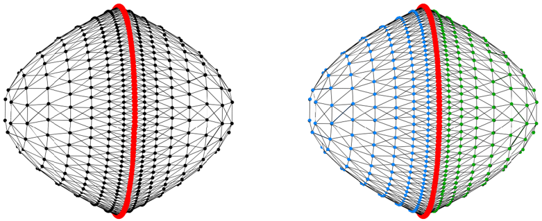
“As part of the construction reviewed in Section 2, the tensor network model provides direct evidence for the existence of the closed universe.”
§ The Baby Universe is Fine and the CFT Knows It: On Holography for Closed Universes > 1.1 FAQ
boosteddirect- Asserted: passes — The authors put it forward as true.
- Checkable: passes — It can be checked against evidence.
- Load-bearing: passes — The paper’s conclusions depend on it.
- Based: passes — The paper gives a reason why it holds.
A conclusion the paper draws from its own results — it cites no other source for it, so there is none to check. The quote shows it is in the paper.
In the paper
“Thus, there is this alternative dual description to |Ψ LR y in terms of two entangled AdS gases in this particular state, as shown in Figure 9.”
§ The Baby Universe is Fine and the CFT Knows It: On Holography for Closed Universes > 3.2.1 Reviewing AR and the EG argument
plaincorrelational- Asserted: passes — The authors put it forward as true.
- Checkable: passes — It can be checked against evidence.
- Load-bearing: passes — The paper’s conclusions depend on it.
- Based: passes — The paper gives a reason why it holds.
A conclusion the paper draws from its own results — it cites no other source for it, so there is none to check. The quote shows it is in the paper.
In the paper
“If we first average over the heavy operators, then the average state has a simple interpretation in terms of quantum field theory on the closed universe.”
§ The Baby Universe is Fine and the CFT Knows It: On Holography for Closed Universes > 1.1 FAQ
plaindirect- Asserted: passes — The authors put it forward as true.
- Checkable: passes — It can be checked against evidence.
- Load-bearing: passes — The paper’s conclusions depend on it.
- Based: passes — The paper gives a reason why it holds.
A conclusion the paper draws from its own results — it cites no other source for it, so there is none to check. The quote shows it is in the paper.
In the paper
“However, in the black hole setup there is no analog of the case where the entanglement with both AdS l and AdS r is small, because the naive bulk entanglement between the interior and Hawking radiation always stays large.”
§ The Baby Universe is Fine and the CFT Knows It: On Holography for Closed Universes > 1.1 FAQ
plain- Asserted: passes — The authors put it forward as true.
- Checkable: passes — It can be checked against evidence.
- Load-bearing: unclear — It is unclear whether the paper’s conclusions depend on it.
- Based: passes — The paper gives a reason why it holds.
A conclusion the paper draws from its own results — it cites no other source for it, so there is none to check. The quote shows it is in the paper.
In the paper
“Taken together, these results amount to a clean bill of health for baby universes born of AdS/CFT.”
§ The Baby Universe is Fine and the CFT Knows It: On Holography for Closed Universes > Abstract
plain- Asserted: passes — The authors put it forward as true.
- Checkable: passes — It can be checked against evidence.
- Load-bearing: passes — The paper’s conclusions depend on it.
- Based: passes — The paper gives a reason why it holds.
The paper states this without a source or data behind it here, so there is nothing to check it against. The quote shows it is in the paper.
In the paper
“This setup-a thermal gas with weak interactions-is a classic dynamical system which exhibits decoherence in the position basis for heavier “probe” particles.”
§ The Baby Universe is Fine and the CFT Knows It: On Holography for Closed Universes > 3.1.1 Comments on observers, pointer variables, and all that
plaindirect- Asserted: passes — The authors put it forward as true.
- Checkable: passes — It can be checked against evidence.
- Load-bearing: unclear — It is unclear whether the paper’s conclusions depend on it.
- Based: unclear — It is unclear why the paper says it holds.
A conclusion the paper draws from its own results — it cites no other source for it, so there is none to check. The quote shows it is in the paper.
In the paper
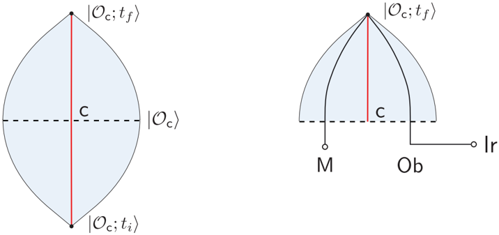
“There is literally a large structure directly related to the CFT state which is interpretable as the space of the closed universe, see Figures 1 and 3.”
§ The Baby Universe is Fine and the CFT Knows It: On Holography for Closed Universes > 1.1 FAQ
boostedcorrelational- Asserted: passes — The authors put it forward as true.
- Checkable: passes — It can be checked against evidence.
- Load-bearing: passes — The paper’s conclusions depend on it.
- Based: passes — The paper gives a reason why it holds.
A conclusion the paper draws from its own results — it cites no other source for it, so there is none to check. The quote shows it is in the paper.
In the paper
“Within this regime, the two parameters mℓ and Eℓ individually determine the coarse-grained entropies of the closed universe and the AdS spaces, respectively.”
§ The Baby Universe is Fine and the CFT Knows It: On Holography for Closed Universes > 2.4 Parameter space in AdS 5 ˆS5
plaindirect- Asserted: passes — The authors put it forward as true.
- Checkable: passes — It can be checked against evidence.
- Load-bearing: passes — The paper’s conclusions depend on it.
- Based: passes — The paper gives a reason why it holds.
A conclusion the paper draws from its own results — it cites no other source for it, so there is none to check. The quote shows it is in the paper.
In the paper
“In particular, we advocate for an interpretation in which the one-dimensional Hilbert space is indicative of the fact that the closed universe is indistinguishable from the outside, e.g. from the perspective of the CFT.”
§ The Baby Universe is Fine and the CFT Knows It: On Holography for Closed Universes > 1.1 FAQ
hedgedcorrelational- Asserted: passes — The authors put it forward as true.
- Checkable: passes — It can be checked against evidence.
- Load-bearing: passes — The paper’s conclusions depend on it.
- Based: unclear — It is unclear why the paper says it holds.
A conclusion the paper draws from its own results — it cites no other source for it, so there is none to check. The quote shows it is in the paper.
In the paper
“We argue that, yes, each element of a suitable ensemble is associated with a closed universe.”
§ The Baby Universe is Fine and the CFT Knows It: On Holography for Closed Universes > 1.1 FAQ
plaincorrelational- Asserted: passes — The authors put it forward as true.
- Checkable: passes — It can be checked against evidence.
- Load-bearing: passes — The paper’s conclusions depend on it.
- Based: passes — The paper gives a reason why it holds.
A conclusion the paper draws from its own results — it cites no other source for it, so there is none to check. The quote shows it is in the paper.
In the paper
“An important difference is that in semiclassical gravity, wormholes swapping closed universes can be important.”
§ The Baby Universe is Fine and the CFT Knows It: On Holography for Closed Universes > 3.2.1 Reviewing AR and the EG argument
plainconditional- Asserted: passes — The authors put it forward as true.
- Checkable: passes — It can be checked against evidence.
- Load-bearing: passes — The paper’s conclusions depend on it.
- Based: unclear — It is unclear why the paper says it holds.
A conclusion the paper draws from its own results — it cites no other source for it, so there is none to check. The quote shows it is in the paper.
In the paper
“In the limit of no bulk entanglement, the holographic encoding breaks down.”
§ The Baby Universe is Fine and the CFT Knows It: On Holography for Closed Universes > Abstract
plaindirect- Asserted: passes — The authors put it forward as true.
- Checkable: passes — It can be checked against evidence.
- Load-bearing: passes — The paper’s conclusions depend on it.
- Based: passes — The paper gives a reason why it holds.
A conclusion the paper draws from its own results — it cites no other source for it, so there is none to check. The quote shows it is in the paper.
In the paper
“The entropy of the bulk state of Hawking radiation in rQFTs is interpreted as the entropy of a coarse-grained or averaged microscopic state, Spρq.”
§ The Baby Universe is Fine and the CFT Knows It: On Holography for Closed Universes > 1.2 Comments on perspectives
plaincorrelational- Asserted: passes — The authors put it forward as true.
- Checkable: passes — It can be checked against evidence.
- Load-bearing: passes — The paper’s conclusions depend on it.
- Based: passes — The paper gives a reason why it holds.
A conclusion the paper draws from its own results — it cites no other source for it, so there is none to check. The quote shows it is in the paper.
In the paper
“The observer-clone setup is at best a “frozen” simulation of what is naturally occurring inside the closed universe.”
§ The Baby Universe is Fine and the CFT Knows It: On Holography for Closed Universes > 3.1.1 Comments on observers, pointer variables, and all that
hedgedcorrelational- Asserted: passes — The authors put it forward as true.
- Checkable: passes — It can be checked against evidence.
- Load-bearing: unclear — It is unclear whether the paper’s conclusions depend on it.
- Based: passes — The paper gives a reason why it holds.
A conclusion the paper draws from its own results — it cites no other source for it, so there is none to check. The quote shows it is in the paper.
In the paper
“This conventional EFT is encoded in CFT data, and it can be probed by computing coarsegrained observables.”
§ The Baby Universe is Fine and the CFT Knows It: On Holography for Closed Universes > Abstract
plaincorrelational- Asserted: passes — The authors put it forward as true.
- Checkable: passes — It can be checked against evidence.
- Load-bearing: passes — The paper’s conclusions depend on it.
- Based: passes — The paper gives a reason why it holds.
None of the sources cited for this claim have been checked yet.
In the paper
“As pointed out in [6], this signals a clear limitation of the conventional holographic encoding of the closed universe as the map W breaks down.”
§ The Baby Universe is Fine and the CFT Knows It: On Holography for Closed Universes > 2.5.3 Highly non-isometric regime
What the sources say
- Not checked yetcites [6] S. Antonini, M. Sasieta and B. Swingle, Cosmology from random entanglement, JHEP 11 (2023) 188 [arXiv:2307.14416] [INSPIRE]. source
Checked before — its earlier verdict is held back until a new check runs.
boosteddirect- Asserted: passes — The authors put it forward as true.
- Checkable: passes — It can be checked against evidence.
- Load-bearing: passes — The paper’s conclusions depend on it.
- Based: passes — The paper gives a reason why it holds.
- Not checked yet
None of the sources cited for this claim have been checked yet.
In the paper
“In this sense, the setup of [6] and discussed here is equivalent to considering the setup of [52] after the cloning procedure has been carried out.”
§ The Baby Universe is Fine and the CFT Knows It: On Holography for Closed Universes > 3.1.1 Comments on observers, pointer variables, and all that
What the sources say
- Not checked yetcites [6] S. Antonini, M. Sasieta and B. Swingle, Cosmology from random entanglement, JHEP 11 (2023) 188 [arXiv:2307.14416] [INSPIRE]. source
Checked before — its earlier verdict is held back until a new check runs.
- Not matchedcites [52] D. Harlow, M. Usatyuk and Y. Zhao, Quantum mechanics and observers for gravity in a closed universe, arXiv:2501.02359 [INSPIRE].
Couldn’t be matched to a paper in Crossref, so it can’t be checked.
plaincorrelational- Asserted: passes — The authors put it forward as true.
- Checkable: passes — It can be checked against evidence.
- Load-bearing: unclear — It is unclear whether the paper’s conclusions depend on it.
- Based: passes — The paper gives a reason why it holds.
- Not checked yet
A conclusion the paper draws from its own results — it cites no other source for it, so there is none to check. The quote shows it is in the paper.
In the paper
“With enough bulk entanglement, the bulk Hilbert space of a closed universe can be holographically encoded in the CFT.”
§ The Baby Universe is Fine and the CFT Knows It: On Holography for Closed Universes > Abstract
plainconditional- Asserted: passes — The authors put it forward as true.
- Checkable: passes — It can be checked against evidence.
- Load-bearing: passes — The paper’s conclusions depend on it.
- Based: passes — The paper gives a reason why it holds.
A conclusion the paper draws from its own results — it cites no other source for it, so there is none to check. The quote shows it is in the paper.
In the paper
“close to this threshold, the entanglement to the universe can be made parametrically large in N , since at the transition point Splrq “ OpN 18{17 q.”
§ The Baby Universe is Fine and the CFT Knows It: On Holography for Closed Universes > 2.4 Parameter space in AdS 5 ˆS5
plaindirect- Asserted: passes — The authors put it forward as true.
- Checkable: passes — It can be checked against evidence.
- Load-bearing: passes — The paper’s conclusions depend on it.
- Based: passes — The paper gives a reason why it holds.
A conclusion the paper draws from its own results — it cites no other source for it, so there is none to check. The quote shows it is in the paper.
In the paper
“Just as in the black hole case, the entropy of the bulk state in rQFTs turns out to be the entropy of a coarse-grained state.”
§ The Baby Universe is Fine and the CFT Knows It: On Holography for Closed Universes > 1.2 Comments on perspectives
plaincorrelational- Asserted: passes — The authors put it forward as true.
- Checkable: passes — It can be checked against evidence.
- Load-bearing: unclear — It is unclear whether the paper’s conclusions depend on it.
- Based: passes — The paper gives a reason why it holds.
None of the sources cited for this claim have been checked yet.
In the paper
“we argue that the physical interpretation of [52] is already implicit in [6] and, indeed, in the structure of EFT more generally.”
§ The Baby Universe is Fine and the CFT Knows It: On Holography for Closed Universes > 1 Introduction
What the sources say
- Not matchedcites [52] D. Harlow, M. Usatyuk and Y. Zhao, Quantum mechanics and observers for gravity in a closed universe, arXiv:2501.02359 [INSPIRE].
Couldn’t be matched to a paper in Crossref, so it can’t be checked.
- Not checked yetcites [6] S. Antonini, M. Sasieta and B. Swingle, Cosmology from random entanglement, JHEP 11 (2023) 188 [arXiv:2307.14416] [INSPIRE]. source
Checked before — its earlier verdict is held back until a new check runs.
plaincorrelational- Asserted: passes — The authors put it forward as true.
- Checkable: passes — It can be checked against evidence.
- Load-bearing: passes — The paper’s conclusions depend on it.
- Based: passes — The paper gives a reason why it holds.
- Not matched
A conclusion the paper draws from its own results — it cites no other source for it, so there is none to check. The quote shows it is in the paper.
In the paper
“We advocate that the CFT nevertheless continues to determine the physical properties of the closed universe in this regime, showing how to interpret this relationship in terms of a final state projection in the closed universe.”
§ The Baby Universe is Fine and the CFT Knows It: On Holography for Closed Universes > Abstract
plaindirect- Asserted: passes — The authors put it forward as true.
- Checkable: passes — It can be checked against evidence.
- Load-bearing: passes — The paper’s conclusions depend on it.
- Based: passes — The paper gives a reason why it holds.
In the paper
“Here we address recent claims made in [60] (referred to in this subsection as EG) and show that their argument against semiclassicality fails.”
§ The Baby Universe is Fine and the CFT Knows It: On Holography for Closed Universes > 3.2 On SWAP tests
What the sources say
- Not matchedcites [60] N. Engelhardt and E. Gesteau, Further Evidence Against a Semiclassical Baby Universe in AdS/CFT, arXiv:2504.14586 [INSPIRE].
Couldn’t be matched to a paper in Crossref, so it can’t be checked.
plain- Asserted: passes — The authors put it forward as true.
- Checkable: passes — It can be checked against evidence.
- Load-bearing: passes — The paper’s conclusions depend on it.
- Based: passes — The paper gives a reason why it holds.
- Not matched
A conclusion the paper draws from its own results — it cites no other source for it, so there is none to check. The quote shows it is in the paper.
In the paper
“Similarly, the entropy computed using rEFTs can be interpreted as a microscopic entropy but averaged over microstates.”
§ The Baby Universe is Fine and the CFT Knows It: On Holography for Closed Universes > 1.2 Comments on perspectives
plaincorrelational- Asserted: passes — The authors put it forward as true.
- Checkable: passes — It can be checked against evidence.
- Load-bearing: unclear — It is unclear whether the paper’s conclusions depend on it.
- Based: passes — The paper gives a reason why it holds.
A conclusion the paper draws from its own results — it cites no other source for it, so there is none to check. The quote shows it is in the paper.
In the paper
“In the effectively isometric regime (blue), the map acts as an approximate isometry for a large collection of bulk states.”
§ The Baby Universe is Fine and the CFT Knows It: On Holography for Closed Universes > 2.5.2 Effectively isometric regime
plaindirect- Asserted: passes — The authors put it forward as true.
- Checkable: passes — It can be checked against evidence.
- Load-bearing: passes — The paper’s conclusions depend on it.
- Based: passes — The paper gives a reason why it holds.
A conclusion the paper draws from its own results — it cites no other source for it, so there is none to check. The quote shows it is in the paper.
In the paper
“Modulo this proviso, we thus expect the internal dynamics of the closed universe to exhibit decoherence in a standard fashion.”
§ The Baby Universe is Fine and the CFT Knows It: On Holography for Closed Universes > 3.1.1 Comments on observers, pointer variables, and all that
hedgedconditional- Asserted: passes — The authors put it forward as true.
- Checkable: passes — It can be checked against evidence.
- Load-bearing: passes — The paper’s conclusions depend on it.
- Based: passes — The paper gives a reason why it holds.
A conclusion the paper draws from its own results — it cites no other source for it, so there is none to check. The quote shows it is in the paper.
In the paper
“If the entanglement with AdS l is large and the entanglement with AdS r is small, the situation is analogous to the black hole near the endpoint of evaporation.”
§ The Baby Universe is Fine and the CFT Knows It: On Holography for Closed Universes > 1.1 FAQ
plaincorrelational- Asserted: passes — The authors put it forward as true.
- Checkable: passes — It can be checked against evidence.
- Load-bearing: unclear — It is unclear whether the paper’s conclusions depend on it.
- Based: passes — The paper gives a reason why it holds.
In the paper
“Moreover, the particular thermal entangled construction we employ has been shown to accurately capture thermal physics [63].”
§ The Baby Universe is Fine and the CFT Knows It: On Holography for Closed Universes > 1.1 FAQ
What the sources say
- Not matchedcites [63] T.J. Sewell, C.D. White and B. Swingle, Thermal Multi-scale Entanglement Renormalization Ansatz for Variational Gibbs State Preparation, arXiv:2210.16419 [INSPIRE].
Couldn’t be matched to a paper in Crossref, so it can’t be checked.
boosteddirect- Asserted: passes — The authors put it forward as true.
- Checkable: passes — It can be checked against evidence.
- Load-bearing: unclear — It is unclear whether the paper’s conclusions depend on it.
- Based: passes — The paper gives a reason why it holds.
- Not matched
A conclusion the paper draws from its own results — it cites no other source for it, so there is none to check. The quote shows it is in the paper.
In the paper
“The oft-cited one-dimensional nature of the closed universe Hilbert space represents the limitation of the external (CFT) Hilbert space to access the quantum information in the closed universe, similar to the limitations imposed on observers outside a perfectly isolated quantum lab.”
§ The Baby Universe is Fine and the CFT Knows It: On Holography for Closed Universes > Abstract
plaindirect- Asserted: passes — The authors put it forward as true.
- Checkable: passes — It can be checked against evidence.
- Load-bearing: passes — The paper’s conclusions depend on it.
- Based: passes — The paper gives a reason why it holds.
A conclusion the paper draws from its own results — it cites no other source for it, so there is none to check. The quote shows it is in the paper.
In the paper
“Once the exact coefficients (given by light-light-heavy OPE coefficients) defining the state |Ψ LR y in this low-energy basis are known, the alternative description can be built simply using the HKLL dictionary and does not manifestly involve a closed universe.”
§ The Baby Universe is Fine and the CFT Knows It: On Holography for Closed Universes > 3.2.1 Reviewing AR and the EG argument
plaindirect- Asserted: passes — The authors put it forward as true.
- Checkable: passes — It can be checked against evidence.
- Load-bearing: passes — The paper’s conclusions depend on it.
- Based: passes — The paper gives a reason why it holds.
A conclusion the paper draws from its own results — it cites no other source for it, so there is none to check. The quote shows it is in the paper.
In the paper
“In the regime where the entanglement with the closed universe is large, the encoding can be obtained via more-or-less conventional tools of entanglement wedge reconstruction, including islands and the like.”
§ The Baby Universe is Fine and the CFT Knows It: On Holography for Closed Universes > 1.1 FAQ
plainconditional- Asserted: passes — The authors put it forward as true.
- Checkable: passes — It can be checked against evidence.
- Load-bearing: passes — The paper’s conclusions depend on it.
- Based: passes — The paper gives a reason why it holds.
A conclusion the paper draws from its own results — it cites no other source for it, so there is none to check. The quote shows it is in the paper.
In the paper
“The main difference between the two setups is in the nature of the bulk representation of entanglement between the two microscopic systems.”
§ The Baby Universe is Fine and the CFT Knows It: On Holography for Closed Universes > 1.1 FAQ
plaincorrelational- Asserted: passes — The authors put it forward as true.
- Checkable: passes — It can be checked against evidence.
- Load-bearing: unclear — It is unclear whether the paper’s conclusions depend on it.
- Based: passes — The paper gives a reason why it holds.
A conclusion the paper draws from its own results — it cites no other source for it, so there is none to check. The quote shows it is in the paper.
In the paper
“In particular, if the entanglement with both AdS l and AdS r is large, this is similar to the interior encoding shortly after the Page time.”
§ The Baby Universe is Fine and the CFT Knows It: On Holography for Closed Universes > 1.1 FAQ
plaincorrelational- Asserted: passes — The authors put it forward as true.
- Checkable: passes — It can be checked against evidence.
- Load-bearing: passes — The paper’s conclusions depend on it.
- Based: passes — The paper gives a reason why it holds.
A conclusion the paper draws from its own results — it cites no other source for it, so there is none to check. The quote shows it is in the paper.
In the paper
“However, this does not mean that individual instances W are likely to be isometric.”
§ The Baby Universe is Fine and the CFT Knows It: On Holography for Closed Universes > 2.5.1 Approximately isometric regime
hedged- Asserted: passes — The authors put it forward as true.
- Checkable: passes — It can be checked against evidence.
- Load-bearing: unclear — It is unclear whether the paper’s conclusions depend on it.
- Based: passes — The paper gives a reason why it holds.
A conclusion the paper draws from its own results — it cites no other source for it, so there is none to check. The quote shows it is in the paper.
In the paper
“for any suitably coarse-grained or averaged property, these erratic amplitudes behave as if they are orthogonal vectors in some larger Hilbert space.”
§ The Baby Universe is Fine and the CFT Knows It: On Holography for Closed Universes > 3.2.4 Interpreting the bulk entanglement
plaincorrelational- Asserted: passes — The authors put it forward as true.
- Checkable: passes — It can be checked against evidence.
- Load-bearing: passes — The paper’s conclusions depend on it.
- Based: passes — The paper gives a reason why it holds.
A conclusion the paper draws from its own results — it cites no other source for it, so there is none to check. The quote shows it is in the paper.
In the paper
“We will propose that the CFT uniquely determines the microscopic structure of the final state of the closed universe.”
§ The Baby Universe is Fine and the CFT Knows It: On Holography for Closed Universes > 4.3 The dictionary
plaindirect- Asserted: passes — The authors put it forward as true.
- Checkable: passes — It can be checked against evidence.
- Load-bearing: passes — The paper’s conclusions depend on it.
- Based: passes — The paper gives a reason why it holds.
A conclusion the paper draws from its own results — it cites no other source for it, so there is none to check. The quote shows it is in the paper.
In the paper
“The one-dimensionality of closed universes represents that from the external observer's Hilbert space (CFT in this case) every closed universe is indistinguishable.”
§ The Baby Universe is Fine and the CFT Knows It: On Holography for Closed Universes > 4.1 The meaning of the one-dimensional Hilbert space
plain- Asserted: passes — The authors put it forward as true.
- Checkable: passes — It can be checked against evidence.
- Load-bearing: passes — The paper’s conclusions depend on it.
- Based: passes — The paper gives a reason why it holds.
A conclusion the paper draws from its own results — it cites no other source for it, so there is none to check. The quote shows it is in the paper.
In the paper
“This shows how the gravitational path integral, and thus the bulk EFT, does not compute the exact microscopic value of the matrix elements, but only their characteristic size over the ensemble.”
§ The Baby Universe is Fine and the CFT Knows It: On Holography for Closed Universes > 5.1 ETH ensemble
boosteddirect- Asserted: passes — The authors put it forward as true.
- Checkable: passes — It can be checked against evidence.
- Load-bearing: passes — The paper’s conclusions depend on it.
- Based: passes — The paper gives a reason why it holds.
- The authors state this as an assumption: The erratic parts of the heavy operator's matrix elements behave as i.i.d. random complex Gaussian variables.
A conclusion the paper draws from its own results — it cites no other source for it, so there is none to check. The quote shows it is in the paper.
In the paper
“In the thermodynamic sense, the final state of the closed universe is a highly entropic state.”
§ The Baby Universe is Fine and the CFT Knows It: On Holography for Closed Universes > 4.3.2 Singularities and quantum chaos
plain- Asserted: passes — The authors put it forward as true.
- Checkable: passes — It can be checked against evidence.
- Load-bearing: unclear — It is unclear whether the paper’s conclusions depend on it.
- Based: passes — The paper gives a reason why it holds.
- The authors state this as an assumption: The erratic parts of the heavy operator's matrix elements behave as i.i.d. random complex Gaussian variables.
A conclusion the paper draws from its own results — it cites no other source for it, so there is none to check. The quote shows it is in the paper.
In the paper
“In this case, the result of the SWAP is controlled by the entanglement entropy between the two CFTs, which in the bulk is captured by the bulk entanglement entropy between fields in the left AdS spacetime and fields in the closed universe.”
§ The Baby Universe is Fine and the CFT Knows It: On Holography for Closed Universes > 3.2.3 How to not swap the closed universes
plaindirect- Asserted: passes — The authors put it forward as true.
- Checkable: passes — It can be checked against evidence.
- Load-bearing: passes — The paper’s conclusions depend on it.
- Based: passes — The paper gives a reason why it holds.
A conclusion the paper draws from its own results — it cites no other source for it, so there is none to check. The quote shows it is in the paper.
In the paper
“The final state wavefunction happens to be very simply related to the microscopic properties of the heavy shell operator.”
§ The Baby Universe is Fine and the CFT Knows It: On Holography for Closed Universes > Figure 14:
plaincorrelational- Asserted: passes — The authors put it forward as true.
- Checkable: passes — It can be checked against evidence.
- Load-bearing: passes — The paper’s conclusions depend on it.
- Based: passes — The paper gives a reason why it holds.
A conclusion the paper draws from its own results — it cites no other source for it, so there is none to check. The quote shows it is in the paper.
In the paper
“Thus, the bulk description is compatible with the ETH ensemble.”
§ The Baby Universe is Fine and the CFT Knows It: On Holography for Closed Universes > 5.1 ETH ensemble
plaincorrelational- Asserted: passes — The authors put it forward as true.
- Checkable: passes — It can be checked against evidence.
- Load-bearing: passes — The paper’s conclusions depend on it.
- Based: passes — The paper gives a reason why it holds.
- The authors state this as an assumption: The erratic parts of the heavy operator's matrix elements behave as i.i.d. random complex Gaussian variables.
A conclusion the paper draws from its own results — it cites no other source for it, so there is none to check. The quote shows it is in the paper.
In the paper
“This permits describing conventional effects such as decoherence and local observers in this framework.”
§ The Baby Universe is Fine and the CFT Knows It: On Holography for Closed Universes > 4.2 Closed universe initial/final state
plaindirect- Asserted: passes — The authors put it forward as true.
- Checkable: passes — It can be checked against evidence.
- Load-bearing: passes — The paper’s conclusions depend on it.
- Based: passes — The paper gives a reason why it holds.
A conclusion the paper draws from its own results — it cites no other source for it, so there is none to check. The quote shows it is in the paper.
In the paper
“The heavy shell in the bulk can be approximated by any of the typical draws of the ensemble.”
§ The Baby Universe is Fine and the CFT Knows It: On Holography for Closed Universes > 5.1 ETH ensemble
plaincorrelational- Asserted: passes — The authors put it forward as true.
- Checkable: passes — It can be checked against evidence.
- Load-bearing: passes — The paper’s conclusions depend on it.
- Based: unclear — It is unclear why the paper says it holds.
- The authors state this as an assumption: The erratic parts of the heavy operator's matrix elements behave as i.i.d. random complex Gaussian variables.
A conclusion the paper draws from its own results — it cites no other source for it, so there is none to check. The quote shows it is in the paper.
In the paper
“Here, this property arises as a consequence of the quantum chaotic features of the CFT.”
§ The Baby Universe is Fine and the CFT Knows It: On Holography for Closed Universes > 4.3.2 Singularities and quantum chaos
plaindirect- Asserted: passes — The authors put it forward as true.
- Checkable: passes — It can be checked against evidence.
- Load-bearing: passes — The paper’s conclusions depend on it.
- Based: passes — The paper gives a reason why it holds.
- The authors state this as an assumption: The erratic parts of the heavy operator's matrix elements behave as i.i.d. random complex Gaussian variables.
A conclusion the paper draws from its own results — it cites no other source for it, so there is none to check. The quote shows it is in the paper.
In the paper
“Some basic properties, such as causality, unitarity, and no-cloning, can be violated at the scale of the universe.”
§ The Baby Universe is Fine and the CFT Knows It: On Holography for Closed Universes > 4.2 Closed universe initial/final state
plainconditional- Asserted: passes — The authors put it forward as true.
- Checkable: passes — It can be checked against evidence.
- Load-bearing: passes — The paper’s conclusions depend on it.
- Based: passes — The paper gives a reason why it holds.
A conclusion the paper draws from its own results — it cites no other source for it, so there is none to check. The quote shows it is in the paper.
In the paper
“As we have seen, as the entanglement between the closed universe and the AdS spacetimes grows, an approximately isometric encoding of the bulk Hilbert space into the dual CFT emerges, (approximately) recovering a more standard holographic dictionary.”
§ The Baby Universe is Fine and the CFT Knows It: On Holography for Closed Universes > 5.3 Reconstructing the closed universe from CFT data
plaindirect- Asserted: passes — The authors put it forward as true.
- Checkable: passes — It can be checked against evidence.
- Load-bearing: passes — The paper’s conclusions depend on it.
- Based: passes — The paper gives a reason why it holds.
- The authors state this as an assumption: The erratic parts of the heavy operator's matrix elements behave as i.i.d. random complex Gaussian variables.
In the paper
“In short, we argue that the SWAP operator discussed in [60], which is supposed to give different results depending on whether or not a closed universe is present, is actually always just the boundary SWAP.”
§ The Baby Universe is Fine and the CFT Knows It: On Holography for Closed Universes > 5.3 Reconstructing the closed universe from CFT data
What the sources say
- Not matchedcites [60] N. Engelhardt and E. Gesteau, Further Evidence Against a Semiclassical Baby Universe in AdS/CFT, arXiv:2504.14586 [INSPIRE].
Couldn’t be matched to a paper in Crossref, so it can’t be checked.
plain- Asserted: passes — The authors put it forward as true.
- Checkable: passes — It can be checked against evidence.
- Load-bearing: passes — The paper’s conclusions depend on it.
- Based: passes — The paper gives a reason why it holds.
- Not matched
A conclusion the paper draws from its own results — it cites no other source for it, so there is none to check. The quote shows it is in the paper.
In the paper
“Global quantum mechanics, on the other hand, is affected by the final state projection, irrespective of the amount of entanglement to the AdS spaces.”
§ The Baby Universe is Fine and the CFT Knows It: On Holography for Closed Universes > 5.3 Reconstructing the closed universe from CFT data
plaindirect- Asserted: passes — The authors put it forward as true.
- Checkable: passes — It can be checked against evidence.
- Load-bearing: passes — The paper’s conclusions depend on it.
- Based: passes — The paper gives a reason why it holds.
A conclusion the paper draws from its own results — it cites no other source for it, so there is none to check. The quote shows it is in the paper.
In the paper
“Both of the rules can be explicitly understood from the CFT doing different experiments with the ensemble of microscopic heavy operators, the difference being whether we correlate draws of the ETH ensemble of operators between different replicas or not.”
§ The Baby Universe is Fine and the CFT Knows It: On Holography for Closed Universes > 5.2.1 Replicas and dimensions
plaindirect- Asserted: passes — The authors put it forward as true.
- Checkable: passes — It can be checked against evidence.
- Load-bearing: passes — The paper’s conclusions depend on it.
- Based: passes — The paper gives a reason why it holds.
- The authors state this as an assumption: The erratic parts of the heavy operator's matrix elements behave as i.i.d. random complex Gaussian variables.
A conclusion the paper draws from its own results — it cites no other source for it, so there is none to check. The quote shows it is in the paper.
In the paper
“The initial state being highly entropic is only a consequence of the symmetry of the setup under time reflection.”
§ The Baby Universe is Fine and the CFT Knows It: On Holography for Closed Universes > 4.3.2 Singularities and quantum chaos
plaindirect- Asserted: passes — The authors put it forward as true.
- Checkable: passes — It can be checked against evidence.
- Load-bearing: unclear — It is unclear whether the paper’s conclusions depend on it.
- Based: passes — The paper gives a reason why it holds.
- The authors state this as an assumption: The erratic parts of the heavy operator's matrix elements behave as i.i.d. random complex Gaussian variables.
A conclusion the paper draws from its own results — it cites no other source for it, so there is none to check. The quote shows it is in the paper.
In the paper
“We have argued that this one-dimensionality simply represents the limitation of the external observer (CFT) to distinguish the quantum information in the closed universe, similar to the limitation of an external observer to describe an isolated quantum lab.”
§ The Baby Universe is Fine and the CFT Knows It: On Holography for Closed Universes > 5.3 Reconstructing the closed universe from CFT data
plaindirect- Asserted: passes — The authors put it forward as true.
- Checkable: passes — It can be checked against evidence.
- Load-bearing: passes — The paper’s conclusions depend on it.
- Based: passes — The paper gives a reason why it holds.
In the paper
“Therefore, the SWAP operator defined in EG cannot detect whether a closed universe is present in the bulk QFT description.”
§ The Baby Universe is Fine and the CFT Knows It: On Holography for Closed Universes > 3.2.2 Addressing the EG argument
What the sources say
- Not matchedcites [60] N. Engelhardt and E. Gesteau, Further Evidence Against a Semiclassical Baby Universe in AdS/CFT, arXiv:2504.14586 [INSPIRE].
Couldn’t be matched to a paper in Crossref, so it can’t be checked.
plain- Asserted: passes — The authors put it forward as true.
- Checkable: passes — It can be checked against evidence.
- Load-bearing: passes — The paper’s conclusions depend on it.
- Based: passes — The paper gives a reason why it holds.
- Rests on an assumption: The standard holographic dictionary and holographic map V apply to the closed universe setup.
- Not matched
A conclusion the paper draws from its own results — it cites no other source for it, so there is none to check. The quote shows it is in the paper.
In the paper
“The [EFT] picture is recovered by performing a correlated average between different replicas for multiple-replica quantities.”
§ The Baby Universe is Fine and the CFT Knows It: On Holography for Closed Universes > 5.3 Reconstructing the closed universe from CFT data
plaindirect- Asserted: passes — The authors put it forward as true.
- Checkable: passes — It can be checked against evidence.
- Load-bearing: passes — The paper’s conclusions depend on it.
- Based: passes — The paper gives a reason why it holds.
A conclusion the paper draws from its own results — it cites no other source for it, so there is none to check. The quote shows it is in the paper.
In the paper
“However, the former (5.3) is a self-consistent [QFT] description in many replicas, without any replica wormholes involved.”
§ The Baby Universe is Fine and the CFT Knows It: On Holography for Closed Universes > 5.2.1 Replicas and dimensions
plain- Asserted: passes — The authors put it forward as true.
- Checkable: passes — It can be checked against evidence.
- Load-bearing: passes — The paper’s conclusions depend on it.
- Based: passes — The paper gives a reason why it holds.
- The authors state this as an assumption: The erratic parts of the heavy operator's matrix elements behave as i.i.d. random complex Gaussian variables.
A conclusion the paper draws from its own results — it cites no other source for it, so there is none to check. The quote shows it is in the paper.
In the paper
“Nevertheless, even in the limit of zero entanglement, the CFT knows about the closed universe in a more general sense.”
§ The Baby Universe is Fine and the CFT Knows It: On Holography for Closed Universes > 3.2.4 Interpreting the bulk entanglement
plain- Asserted: passes — The authors put it forward as true.
- Checkable: passes — It can be checked against evidence.
- Load-bearing: passes — The paper’s conclusions depend on it.
- Based: passes — The paper gives a reason why it holds.
A conclusion the paper draws from its own results — it cites no other source for it, so there is none to check. The quote shows it is in the paper.
In the paper
“From the CFT perspective, the statistics is taken over an ensemble of heavy microscopic operators compatible with the heavy shell, whose light matrix elements behave erratically.”
§ The Baby Universe is Fine and the CFT Knows It: On Holography for Closed Universes > 5.3 Reconstructing the closed universe from CFT data
plaincorrelational- Asserted: passes — The authors put it forward as true.
- Checkable: passes — It can be checked against evidence.
- Load-bearing: passes — The paper’s conclusions depend on it.
- Based: passes — The paper gives a reason why it holds.
A conclusion the paper draws from its own results — it cites no other source for it, so there is none to check. The quote shows it is in the paper.
In the paper
“The statistics of the results of experiments in the CFT can in turn be used to deduce properties of the closed universe.”
§ The Baby Universe is Fine and the CFT Knows It: On Holography for Closed Universes > 5.3 Reconstructing the closed universe from CFT data
plaindirect- Asserted: passes — The authors put it forward as true.
- Checkable: passes — It can be checked against evidence.
- Load-bearing: passes — The paper’s conclusions depend on it.
- Based: passes — The paper gives a reason why it holds.
- The authors state this as an assumption: The erratic parts of the heavy operator's matrix elements behave as i.i.d. random complex Gaussian variables.
A conclusion the paper draws from its own results — it cites no other source for it, so there is none to check. The quote shows it is in the paper.
In the paper
“The expectation value xgs|O piq |gsy can be probed by a boundary CFT experiment using the following protocol.”
§ The Baby Universe is Fine and the CFT Knows It: On Holography for Closed Universes > 5.3 Reconstructing the closed universe from CFT data
plaindirect- Asserted: passes — The authors put it forward as true.
- Checkable: passes — It can be checked against evidence.
- Load-bearing: passes — The paper’s conclusions depend on it.
- Based: passes — The paper gives a reason why it holds.
- The authors state this as an assumption: The erratic parts of the heavy operator's matrix elements behave as i.i.d. random complex Gaussian variables.
A conclusion the paper draws from its own results — it cites no other source for it, so there is none to check. The quote shows it is in the paper.
In the paper
“From the Hilbert space of the CFT, two microstates representing different states of the universe become indistinguishable, as they are exactly parallel quantum states.”
§ The Baby Universe is Fine and the CFT Knows It: On Holography for Closed Universes > 4.1 The meaning of the one-dimensional Hilbert space
plain- Asserted: passes — The authors put it forward as true.
- Checkable: passes — It can be checked against evidence.
- Load-bearing: passes — The paper’s conclusions depend on it.
- Based: passes — The paper gives a reason why it holds.
None of the sources cited for this claim have been checked yet.
In the paper
“In particular, we have argued that the model presented in [52], which relies on the definition of an”
§ The Baby Universe is Fine and the CFT Knows It: On Holography for Closed Universes > 5.3 Reconstructing the closed universe from CFT data
What the sources say
- Not matchedcites [52] D. Harlow, M. Usatyuk and Y. Zhao, Quantum mechanics and observers for gravity in a closed universe, arXiv:2501.02359 [INSPIRE].
Couldn’t be matched to a paper in Crossref, so it can’t be checked.
- Not checked yetcites [6] S. Antonini, M. Sasieta and B. Swingle, Cosmology from random entanglement, JHEP 11 (2023) 188 [arXiv:2307.14416] [INSPIRE]. source
Checked before — its earlier verdict is held back until a new check runs.
plaincorrelational- Asserted: passes — The authors put it forward as true.
- Checkable: passes — It can be checked against evidence.
- Load-bearing: unclear — It is unclear whether the paper’s conclusions depend on it.
- Based: passes — The paper gives a reason why it holds.
- Not matched
A conclusion the paper draws from its own results — it cites no other source for it, so there is none to check. The quote shows it is in the paper.
In the paper
“The holographic map is then a Heisenberg picture model of such a projection, where the final state has been suitably propagated to the time-symmetric slice of the universe using the Hamiltonian defined by the background, as shown in Figure 13.”
§ The Baby Universe is Fine and the CFT Knows It: On Holography for Closed Universes > 4.2 Closed universe initial/final state
plaindirect- Asserted: passes — The authors put it forward as true.
- Checkable: passes — It can be checked against evidence.
- Load-bearing: passes — The paper’s conclusions depend on it.
- Based: passes — The paper gives a reason why it holds.
- Rests on an assumption: The standard holographic dictionary and holographic map V apply to the closed universe setup.
A conclusion the paper draws from its own results — it cites no other source for it, so there is none to check. The quote shows it is in the paper.
In the paper
“In this section, we will show that the conventional global EFT of the closed universe, without any final state projection, can still be described from the CFT if one chooses to implement an average over the microscopics of the final state.”
§ The Baby Universe is Fine and the CFT Knows It: On Holography for Closed Universes > 4.4 Arrow of time
plainconditional- Asserted: passes — The authors put it forward as true.
- Checkable: passes — It can be checked against evidence.
- Load-bearing: passes — The paper’s conclusions depend on it.
- Based: passes — The paper gives a reason why it holds.
- The authors state this as an assumption: The erratic parts of the heavy operator's matrix elements behave as i.i.d. random complex Gaussian variables.
A conclusion the paper draws from its own results — it cites no other source for it, so there is none to check. The quote shows it is in the paper.
In the paper
“The specific state |O c y the map projects the closed universe onto was defined after (2.7) and it depends on the microscopics of the heavy CFT operator used to create the shell.”
§ The Baby Universe is Fine and the CFT Knows It: On Holography for Closed Universes > 4.2 Closed universe initial/final state
plaindirect- Asserted: passes — The authors put it forward as true.
- Checkable: passes — It can be checked against evidence.
- Load-bearing: unclear — It is unclear whether the paper’s conclusions depend on it.
- Based: passes — The paper gives a reason why it holds.
A conclusion the paper draws from its own results — it cites no other source for it, so there is none to check. The quote shows it is in the paper.
In the paper
“From the point of view of the holographic map, the projection in this regime is the extreme non-isometric case discussed in Section 2.”
§ The Baby Universe is Fine and the CFT Knows It: On Holography for Closed Universes > 4.2 Closed universe initial/final state
plaincorrelational- Asserted: passes — The authors put it forward as true.
- Checkable: passes — It can be checked against evidence.
- Load-bearing: passes — The paper’s conclusions depend on it.
- Based: passes — The paper gives a reason why it holds.
- Rests on an assumption: The standard holographic dictionary and holographic map V apply to the closed universe setup.
None of the sources cited for this claim have been checked yet.
In the paper
“Well-known arguments [52,53,109,111] indicate that the Hilbert space of the closed universe is one-dimensional in this regime.”
§ The Baby Universe is Fine and the CFT Knows It: On Holography for Closed Universes > 5.3 Reconstructing the closed universe from CFT data
What the sources say
- Not matchedcites [52] D. Harlow, M. Usatyuk and Y. Zhao, Quantum mechanics and observers for gravity in a closed universe, arXiv:2501.02359 [INSPIRE].
Couldn’t be matched to a paper in Crossref, so it can’t be checked.
- Not checked yetcites [53] A.I. Abdalla, S. Antonini, L.V. Iliesiu and A. Levine, The gravitational path integral from an observer’s point of view, JHEP 05 (2025) 059 [arXiv:2501.02632] [INSPIRE]. source
Checked before — its earlier verdict is held back until a new check runs.
- Not matchedcites [109] J. McNamara and C. Vafa, Cobordism Classes and the Swampland, arXiv:1909.10355 [INSPIRE].
Couldn’t be matched to a paper in Crossref, so it can’t be checked.
- Not checked yetcites [111] D. Marolf and H. Maxfield, Transcending the ensemble: baby universes, spacetime wormholes, and the order and disorder of black hole information, JHEP 08 (2020) 044 [arXiv:2002.08950] [INSPIRE]. source
boosted- Asserted: passes — The authors put it forward as true.
- Checkable: passes — It can be checked against evidence.
- Load-bearing: passes — The paper’s conclusions depend on it.
- Based: passes — The paper gives a reason why it holds.
- Not matched
A conclusion the paper draws from its own results — it cites no other source for it, so there is none to check. The quote shows it is in the paper.
In the paper
“If we coarse-grain in the way the gravitational path integral does, we lose information about the specific final state.”
§ The Baby Universe is Fine and the CFT Knows It: On Holography for Closed Universes > 5.2.2 Connection to α-states in a many-universe Hilbert space
plaindirect- Asserted: passes — The authors put it forward as true.
- Checkable: passes — It can be checked against evidence.
- Load-bearing: passes — The paper’s conclusions depend on it.
- Based: passes — The paper gives a reason why it holds.
- The authors state this as an assumption: The erratic parts of the heavy operator's matrix elements behave as i.i.d. random complex Gaussian variables.
A conclusion the paper draws from its own results — it cites no other source for it, so there is none to check. The quote shows it is in the paper.
In the paper
“We remark that the statistical properties of this ensemble can be deduced directly from CFT experiments:”
§ The Baby Universe is Fine and the CFT Knows It: On Holography for Closed Universes > 5.3 Reconstructing the closed universe from CFT data
plaindirect- Asserted: passes — The authors put it forward as true.
- Checkable: passes — It can be checked against evidence.
- Load-bearing: passes — The paper’s conclusions depend on it.
- Based: passes — The paper gives a reason why it holds.
- The authors state this as an assumption: The erratic parts of the heavy operator's matrix elements behave as i.i.d. random complex Gaussian variables.
In the paper
“The breakdown of semiclassicality advocated for in [60] follows only if the CFT inner product, which is not well-approximated by the bulk [QFT] in the regime of small entanglement, is the one relevant for the description of ordinary physics in the closed universe.”
§ The Baby Universe is Fine and the CFT Knows It: On Holography for Closed Universes > 5.3 Reconstructing the closed universe from CFT data
What the sources say
- Not matchedcites [60] N. Engelhardt and E. Gesteau, Further Evidence Against a Semiclassical Baby Universe in AdS/CFT, arXiv:2504.14586 [INSPIRE].
Couldn’t be matched to a paper in Crossref, so it can’t be checked.
plainconditional- Asserted: passes — The authors put it forward as true.
- Checkable: passes — It can be checked against evidence.
- Load-bearing: passes — The paper’s conclusions depend on it.
- Based: passes — The paper gives a reason why it holds.
- Not matched
A conclusion the paper draws from its own results — it cites no other source for it, so there is none to check. The quote shows it is in the paper.
In the paper
“we show that the presence of both initial and final state projections has an interesting implication for the arrow of time.”
§ The Baby Universe is Fine and the CFT Knows It: On Holography for Closed Universes > 4.4 Arrow of time
plaindirect- Asserted: passes — The authors put it forward as true.
- Checkable: passes — It can be checked against evidence.
- Load-bearing: passes — The paper’s conclusions depend on it.
- Based: passes — The paper gives a reason why it holds.
A conclusion the paper draws from its own results — it cites no other source for it, so there is none to check. The quote shows it is in the paper.
In the paper
“However, as we noted above, the one-dimensionality of the closed universe Hilbert space, suitably defined, is a prediction of rEFTs.”
§ The Baby Universe is Fine and the CFT Knows It: On Holography for Closed Universes > 3.2.5 Closing comments
plaindirect- Asserted: passes — The authors put it forward as true.
- Checkable: passes — It can be checked against evidence.
- Load-bearing: passes — The paper’s conclusions depend on it.
- Based: unclear — It is unclear why the paper says it holds.
A conclusion the paper draws from its own results — it cites no other source for it, so there is none to check. The quote shows it is in the paper.
In the paper
“A state-dependent reconstruction of the [QFT] in the closed universe background is possible using this encoding.”
§ The Baby Universe is Fine and the CFT Knows It: On Holography for Closed Universes > 5.3 Reconstructing the closed universe from CFT data
hedgeddirect- Asserted: passes — The authors put it forward as true.
- Checkable: passes — It can be checked against evidence.
- Load-bearing: passes — The paper’s conclusions depend on it.
- Based: passes — The paper gives a reason why it holds.
A conclusion the paper draws from its own results — it cites no other source for it, so there is none to check. The quote shows it is in the paper.
In the paper
“Taking this perspective, the final state projection modifies the global structure of the quantum mechanics in the closed universe, irrespective of whether there is entanglement with the exterior or not.”
§ The Baby Universe is Fine and the CFT Knows It: On Holography for Closed Universes > 4.2 Closed universe initial/final state
plaindirect- Asserted: passes — The authors put it forward as true.
- Checkable: passes — It can be checked against evidence.
- Load-bearing: passes — The paper’s conclusions depend on it.
- Based: passes — The paper gives a reason why it holds.
- Rests on an assumption: The final state projection perspective is a valid model of the closed universe.
None of the sources cited for this claim have been checked yet.
In the paper
“The heavy operator O is expected to have erratic matrix elements between light states of the CFT.”
§ The Baby Universe is Fine and the CFT Knows It: On Holography for Closed Universes > 4.3.2 Singularities and quantum chaos
What the sources say
- Not checked yetcites [84] A. Belin and J. de Boer, Random statistics of OPE coefficients and Euclidean wormholes, Class. Quant. Grav. 38 (2021) 164001 [arXiv:2006.05499] [INSPIRE]. source
Checked before — its earlier verdict is held back until a new check runs.
- Not checked — no full text of the sourcecites [120] M. Srednicki, Chaos and Quantum Thermalization, Phys. Rev. E 50 (1994) 888 [cond-mat/9403051] [INSPIRE]. source
- Not checked yetcites [121] S. Collier, A. Maloney, H. Maxfield and I. Tsiares, Universal dynamics of heavy operators in CFT2, JHEP 07 (2020) 074 [arXiv:1912.00222] [INSPIRE]. source
Checked before — its earlier verdict is held back until a new check runs.
hedgedcorrelational- Asserted: passes — The authors put it forward as true.
- Checkable: passes — It can be checked against evidence.
- Load-bearing: passes — The paper’s conclusions depend on it.
- Based: passes — The paper gives a reason why it holds.
- The authors state this as an assumption: The erratic parts of the heavy operator's matrix elements behave as i.i.d. random complex Gaussian variables.
- Not checked yet
A conclusion the paper draws from its own results — it cites no other source for it, so there is none to check. The quote shows it is in the paper.
In the paper
“The intrinsic closed universe-to-CFT dictionary suggested by (4.3) is thus: final state wavefunction Ø CFT light-light matrix elements of O Ψ I O”
§ The Baby Universe is Fine and the CFT Knows It: On Holography for Closed Universes > Figure 14:
hedgedcorrelational- Asserted: passes — The authors put it forward as true.
- Checkable: passes — It can be checked against evidence.
- Load-bearing: passes — The paper’s conclusions depend on it.
- Based: passes — The paper gives a reason why it holds.
A conclusion the paper draws from its own results — it cites no other source for it, so there is none to check. The quote shows it is in the paper.
In the paper
“An interesting fact is that this concrete proposal connects the quantum structure of singularities to the chaotic features of the CFT.”
§ The Baby Universe is Fine and the CFT Knows It: On Holography for Closed Universes > 4.3.2 Singularities and quantum chaos
plaincorrelational- Asserted: passes — The authors put it forward as true.
- Checkable: passes — It can be checked against evidence.
- Load-bearing: passes — The paper’s conclusions depend on it.
- Based: passes — The paper gives a reason why it holds.
A conclusion the paper draws from its own results — it cites no other source for it, so there is none to check. The quote shows it is in the paper.
In the paper
“If instead we perform a correlated average for all the copies, we can access the average value of non-linear quantities depending on the final state ρ.”
§ The Baby Universe is Fine and the CFT Knows It: On Holography for Closed Universes > 5.2.1 Replicas and dimensions
plaindirect- Asserted: passes — The authors put it forward as true.
- Checkable: passes — It can be checked against evidence.
- Load-bearing: passes — The paper’s conclusions depend on it.
- Based: passes — The paper gives a reason why it holds.
- The authors state this as an assumption: The erratic parts of the heavy operator's matrix elements behave as i.i.d. random complex Gaussian variables.
None of the sources cited for this claim have been checked yet.
In the paper
“are reproduced by spacetime wormhole contributions to moments of the matrix elements of the shell operator [76].”
§ The Baby Universe is Fine and the CFT Knows It: On Holography for Closed Universes > 4.3.2 Singularities and quantum chaos
What the sources say
- Not checked yetcites [76] M. Sasieta, Wormholes from heavy operator statistics in AdS/CFT, JHEP 03 (2023) 158 [arXiv:2211.11794] [INSPIRE]. source
Checked before — its earlier verdict is held back until a new check runs.
plaindirect- Asserted: passes — The authors put it forward as true.
- Checkable: passes — It can be checked against evidence.
- Load-bearing: passes — The paper’s conclusions depend on it.
- Based: passes — The paper gives a reason why it holds.
- The authors state this as an assumption: The erratic parts of the heavy operator's matrix elements behave as i.i.d. random complex Gaussian variables.
- Not checked yet
None of the sources cited for this claim have been checked yet.
In the paper
“When the entanglement entropy is sufficiently large, the situation is a rather conventional encoding, analogous to the situation for the black hole interior [68].”
§ The Baby Universe is Fine and the CFT Knows It: On Holography for Closed Universes > 5.3 Reconstructing the closed universe from CFT data
What the sources say
- Not checked yetcites [68] C. Akers et al., The black hole interior from non-isometric codes and complexity, JHEP 06 (2024) 155 [arXiv:2207.06536] [INSPIRE]. source
Checked before — its earlier verdict is held back until a new check runs.
plainconditional- Asserted: passes — The authors put it forward as true.
- Checkable: passes — It can be checked against evidence.
- Load-bearing: passes — The paper’s conclusions depend on it.
- Based: passes — The paper gives a reason why it holds.
- Not checked yet
A conclusion the paper draws from its own results — it cites no other source for it, so there is none to check. The quote shows it is in the paper.
In the paper
“The difference is that the bulk state of the quantum fields gets always projected into the fixed state |O c y in the universe, instead of traced over states in c.”
§ The Baby Universe is Fine and the CFT Knows It: On Holography for Closed Universes > 4.2 Closed universe initial/final state
plaindirect- Asserted: passes — The authors put it forward as true.
- Checkable: passes — It can be checked against evidence.
- Load-bearing: passes — The paper’s conclusions depend on it.
- Based: passes — The paper gives a reason why it holds.
- Rests on an assumption: The standard holographic dictionary and holographic map V apply to the closed universe setup.
None of the sources cited for this claim have been checked yet.
In the paper
“The situation with the closed universe is essentially the same, right down to the erratic/random nature of the states [6].”
§ The Baby Universe is Fine and the CFT Knows It: On Holography for Closed Universes > 3.2.4 Interpreting the bulk entanglement
What the sources say
- Not checked yetcites [6] S. Antonini, M. Sasieta and B. Swingle, Cosmology from random entanglement, JHEP 11 (2023) 188 [arXiv:2307.14416] [INSPIRE]. source
Checked before — its earlier verdict is held back until a new check runs.
plaincorrelational- Asserted: passes — The authors put it forward as true.
- Checkable: passes — It can be checked against evidence.
- Load-bearing: unclear — It is unclear whether the paper’s conclusions depend on it.
- Based: passes — The paper gives a reason why it holds.
- Rests on an assumption: In gravitating systems, fine-grained entropies of microscopic systems can be captured in terms of coarse-grained entropies of dynamically determined regions of the geometry.
- Not checked yet
In the paper
“Because the causal wedge SWAP, when mapped to the CFT using the holographic map, is just the boundary SWAP, it also swaps the closed universes.”
- Also stated in: § 3.2.5 Closing comments · plain
“Reflecting back on the analysis in this section, we argued that the causal wedge SWAP described by EG is simply the boundary SWAP and the result of such a SWAP test on the CFT state is unit purity.”
§ The Baby Universe is Fine and the CFT Knows It: On Holography for Closed Universes > 3.2.2 Addressing the EG argument
What the sources say
- Not matchedcites [60] N. Engelhardt and E. Gesteau, Further Evidence Against a Semiclassical Baby Universe in AdS/CFT, arXiv:2504.14586 [INSPIRE].
Couldn’t be matched to a paper in Crossref, so it can’t be checked.
plain- Asserted: passes — The authors put it forward as true.
- Checkable: passes — It can be checked against evidence.
- Load-bearing: passes — The paper’s conclusions depend on it.
- Based: passes — The paper gives a reason why it holds.
- Rests on an assumption: The standard holographic dictionary and holographic map V apply to the closed universe setup.
- Also stated in: § 3.2.5 Closing comments · plain
A conclusion the paper draws from its own results — it cites no other source for it, so there is none to check. The quote shows it is in the paper.
In the paper
“Now the same bulk QFT SWAP on the l bulk fields, which still maps to the L CFT SWAP, does not SWAP the closed universes, as shown in Figure 11 with L and R interchanged.”
§ The Baby Universe is Fine and the CFT Knows It: On Holography for Closed Universes > 3.2.3 How to not swap the closed universes
plain- Asserted: passes — The authors put it forward as true.
- Checkable: passes — It can be checked against evidence.
- Load-bearing: passes — The paper’s conclusions depend on it.
- Based: passes — The paper gives a reason why it holds.
A conclusion the paper draws from its own results — it cites no other source for it, so there is none to check. The quote shows it is in the paper.
In the paper
“We emphasize that the”
§ The Baby Universe is Fine and the CFT Knows It: On Holography for Closed Universes > 3.2.4 Interpreting the bulk entanglement
plain- Asserted: passes — The authors put it forward as true.
- Checkable: passes — It can be checked against evidence.
- Load-bearing: passes — The paper’s conclusions depend on it.
- Based: passes — The paper gives a reason why it holds.
A claim is checked only against the cited paper’s full text, never its abstract, and none is available for its sources.
In the paper
“Still, restricting to sufficiently local subsystems, one expects to recover conventional quantum mechanics without any projection [104,116].”
§ The Baby Universe is Fine and the CFT Knows It: On Holography for Closed Universes > 4.2 Closed universe initial/final state
What the sources say
- Not checked — no full text of the sourcecites [104] G.T. Horowitz and J.M. Maldacena, The black hole final state, JHEP 02 (2004) 008 [hep-th/0310281] [INSPIRE]. source
- Not checked — no full text of the sourcecites [116] S. Lloyd and J. Preskill, Unitarity of black hole evaporation in final-state projection models, JHEP 08 (2014) 126 [arXiv:1308.4209] [INSPIRE]. source
hedgedconditional- Asserted: passes — The authors put it forward as true.
- Checkable: passes — It can be checked against evidence.
- Load-bearing: passes — The paper’s conclusions depend on it.
- Based: passes — The paper gives a reason why it holds.
A conclusion the paper draws from its own results — it cites no other source for it, so there is none to check. The quote shows it is in the paper.
In the paper
“By post-selecting specific measurement outcomes that single out a consistent microstate and conveying this information to the L CFT, one can select a corresponding subset of the SWAP test outcomes for which the two states in the SWAP test happened to agree, and that subset of the data will give an estimate of unit purity.”
§ The Baby Universe is Fine and the CFT Knows It: On Holography for Closed Universes > 3.2.3 How to not swap the closed universes
plaindirect- Asserted: passes — The authors put it forward as true.
- Checkable: passes — It can be checked against evidence.
- Load-bearing: passes — The paper’s conclusions depend on it.
- Based: passes — The paper gives a reason why it holds.
A conclusion the paper draws from its own results — it cites no other source for it, so there is none to check. The quote shows it is in the paper.
In the paper
“In the regime in which the bulk entanglement is largest between the closed universe and the r bulk fields, the closed universe is in the entanglement wedge of the r bulk fields (and the R CFT) and not the L CFT.”
§ The Baby Universe is Fine and the CFT Knows It: On Holography for Closed Universes > 3.2.3 How to not swap the closed universes
plaincorrelational- Asserted: passes — The authors put it forward as true.
- Checkable: passes — It can be checked against evidence.
- Load-bearing: passes — The paper’s conclusions depend on it.
- Based: passes — The paper gives a reason why it holds.
- Rests on an assumption: The standard holographic dictionary and holographic map V apply to the closed universe setup.
A conclusion the paper draws from its own results — it cites no other source for it, so there is none to check. The quote shows it is in the paper.
In the paper
“the Schrodinger's cat like ground state, being a consequence of discrete symmetry breaking, should be stable to any small perturbation of H SC that respects the symmetry.”
§ The Baby Universe is Fine and the CFT Knows It: On Holography for Closed Universes > 4.4 Arrow of time
plaindirect- Asserted: passes — The authors put it forward as true.
- Checkable: passes — It can be checked against evidence.
- Load-bearing: unclear — It is unclear whether the paper’s conclusions depend on it.
- Based: passes — The paper gives a reason why it holds.
- The authors state this as an assumption: The system Hamiltonian H is a random GOE matrix.
- The authors state this as an assumption: The CR action is trivial.
- The authors state this as an assumption: The system and clock are non-interacting.
A conclusion the paper draws from its own results — it cites no other source for it, so there is none to check. The quote shows it is in the paper.
In the paper
“From the bulk point of view, this can be interpreted as saying that conventional EFT, ignoring final state projections at terminal spacelike singularities, is equivalent to the maximally ignorant description of the final state.”
§ The Baby Universe is Fine and the CFT Knows It: On Holography for Closed Universes > 4.4 Arrow of time
plaincorrelational- Asserted: passes — The authors put it forward as true.
- Checkable: passes — It can be checked against evidence.
- Load-bearing: passes — The paper’s conclusions depend on it.
- Based: passes — The paper gives a reason why it holds.
- The authors state this as an assumption: The erratic parts of the heavy operator's matrix elements behave as i.i.d. random complex Gaussian variables.
A conclusion the paper draws from its own results — it cites no other source for it, so there is none to check. The quote shows it is in the paper.
In the paper
“This leads to natural closed universe tensor network representations of the matrix elements (4.3), as shown in Figure 14.”
§ The Baby Universe is Fine and the CFT Knows It: On Holography for Closed Universes > 4.3 The dictionary
plaindirect- Asserted: passes — The authors put it forward as true.
- Checkable: passes — It can be checked against evidence.
- Load-bearing: unclear — It is unclear whether the paper’s conclusions depend on it.
- Based: passes — The paper gives a reason why it holds.
- Rests on an assumption: The tensor network model used faithfully represents the relevant CFT/closed universe physics.
A conclusion the paper draws from its own results — it cites no other source for it, so there is none to check. The quote shows it is in the paper.
In the paper
“We thus obtain the averaged two-point function Gpαq purely from the statistics of CFT experiments.”
§ The Baby Universe is Fine and the CFT Knows It: On Holography for Closed Universes > 5.3 Reconstructing the closed universe from CFT data
plaindirect- Asserted: passes — The authors put it forward as true.
- Checkable: passes — It can be checked against evidence.
- Load-bearing: passes — The paper’s conclusions depend on it.
- Based: passes — The paper gives a reason why it holds.
- The authors state this as an assumption: The erratic parts of the heavy operator's matrix elements behave as i.i.d. random complex Gaussian variables.
A conclusion the paper draws from its own results — it cites no other source for it, so there is none to check. The quote shows it is in the paper.
In the paper
“We argued that the difference, as signaled by the holographic encoding, is that there is a final state projection implemented in the universe.”
§ The Baby Universe is Fine and the CFT Knows It: On Holography for Closed Universes > 5.3 Reconstructing the closed universe from CFT data
plaincorrelational- Asserted: passes — The authors put it forward as true.
- Checkable: passes — It can be checked against evidence.
- Load-bearing: passes — The paper’s conclusions depend on it.
- Based: passes — The paper gives a reason why it holds.
A conclusion the paper draws from its own results — it cites no other source for it, so there is none to check. The quote shows it is in the paper.
In the paper
“It is worth emphasizing at this point that the final state projection is compatible with the reconstruction of operators in the closed universe via the non-isometric encoding when sufficient entanglement with exterior regions is present.”
§ The Baby Universe is Fine and the CFT Knows It: On Holography for Closed Universes > 5.3 Reconstructing the closed universe from CFT data
plainconditional- Asserted: passes — The authors put it forward as true.
- Checkable: passes — It can be checked against evidence.
- Load-bearing: passes — The paper’s conclusions depend on it.
- Based: passes — The paper gives a reason why it holds.
A conclusion the paper draws from its own results — it cites no other source for it, so there is none to check. The quote shows it is in the paper.
In the paper
“The Gaussian integral over microscopic matrix elements O I can be reinterpreted in the language of a Hilbert space of bosonic excitations.”
§ The Baby Universe is Fine and the CFT Knows It: On Holography for Closed Universes > 5.2.2 Connection to α-states in a many-universe Hilbert space
plaincorrelational- Asserted: passes — The authors put it forward as true.
- Checkable: passes — It can be checked against evidence.
- Load-bearing: passes — The paper’s conclusions depend on it.
- Based: passes — The paper gives a reason why it holds.
- The authors state this as an assumption: The erratic parts of the heavy operator's matrix elements behave as i.i.d. random complex Gaussian variables.
A conclusion the paper draws from its own results — it cites no other source for it, so there is none to check. The quote shows it is in the paper.
In the paper
“Notice that by increasing α, we can probe regions further from the shell, all the way to the center of the closed universe in the limit α Ñ 8.”
§ The Baby Universe is Fine and the CFT Knows It: On Holography for Closed Universes > 5.3 Reconstructing the closed universe from CFT data
plaindirect- Asserted: passes — The authors put it forward as true.
- Checkable: passes — It can be checked against evidence.
- Load-bearing: passes — The paper’s conclusions depend on it.
- Based: passes — The paper gives a reason why it holds.
- The authors state this as an assumption: The erratic parts of the heavy operator's matrix elements behave as i.i.d. random complex Gaussian variables.
None of the sources cited for this claim have been checked yet.
In the paper
“The specific structure of these matrix elements can be viewed as a generalized version of the eigenstate thermalization hypothesis (ETH) [84,120,121].”
§ The Baby Universe is Fine and the CFT Knows It: On Holography for Closed Universes > 4.3.2 Singularities and quantum chaos
What the sources say
- Not checked yetcites [84] A. Belin and J. de Boer, Random statistics of OPE coefficients and Euclidean wormholes, Class. Quant. Grav. 38 (2021) 164001 [arXiv:2006.05499] [INSPIRE]. source
Checked before — its earlier verdict is held back until a new check runs.
- Not checked — no full text of the sourcecites [120] M. Srednicki, Chaos and Quantum Thermalization, Phys. Rev. E 50 (1994) 888 [cond-mat/9403051] [INSPIRE]. source
- Not checked yetcites [121] S. Collier, A. Maloney, H. Maxfield and I. Tsiares, Universal dynamics of heavy operators in CFT2, JHEP 07 (2020) 074 [arXiv:1912.00222] [INSPIRE]. source
Checked before — its earlier verdict is held back until a new check runs.
plaincorrelational- Asserted: passes — The authors put it forward as true.
- Checkable: passes — It can be checked against evidence.
- Load-bearing: unclear — It is unclear whether the paper’s conclusions depend on it.
- Based: passes — The paper gives a reason why it holds.
- The authors state this as an assumption: The erratic parts of the heavy operator's matrix elements behave as i.i.d. random complex Gaussian variables.
- Not checked yet
A conclusion the paper draws from its own results — it cites no other source for it, so there is none to check. The quote shows it is in the paper.
In the paper
“From the external observer (the CFT) the conclusion would still be the same: in the regime of no entanglement, all of the universes are indistinguishable and thus the external Hilbert space describing them is one-dimensional.”
§ The Baby Universe is Fine and the CFT Knows It: On Holography for Closed Universes > 4.1 The meaning of the one-dimensional Hilbert space
hedgeddirect- Asserted: passes — The authors put it forward as true.
- Checkable: passes — It can be checked against evidence.
- Load-bearing: passes — The paper’s conclusions depend on it.
- Based: passes — The paper gives a reason why it holds.
A conclusion the paper draws from its own results — it cites no other source for it, so there is none to check. The quote shows it is in the paper.
In the paper
“We advocated this is not the case, and interpreted instead the large fluctuations (at low entanglement) in the [QFT] approximation of the CFT inner product as a breakdown of the ordinary holographic encoding of the closed universe.”
§ The Baby Universe is Fine and the CFT Knows It: On Holography for Closed Universes > 5.3 Reconstructing the closed universe from CFT data
plaindirect- Asserted: passes — The authors put it forward as true.
- Checkable: passes — It can be checked against evidence.
- Load-bearing: passes — The paper’s conclusions depend on it.
- Based: passes — The paper gives a reason why it holds.
A conclusion the paper draws from its own results — it cites no other source for it, so there is none to check. The quote shows it is in the paper.
In the paper
“This is an operator that effectively SWAPs the state of the particle in AdS but not the state of the particle in the closed universe.”
§ The Baby Universe is Fine and the CFT Knows It: On Holography for Closed Universes > 3.2.3 How to not swap the closed universes
plaindirect- Asserted: passes — The authors put it forward as true.
- Checkable: passes — It can be checked against evidence.
- Load-bearing: passes — The paper’s conclusions depend on it.
- Based: passes — The paper gives a reason why it holds.
A conclusion the paper draws from its own results — it cites no other source for it, so there is none to check. The quote shows it is in the paper.
In the paper
“For example, considering the statistical properties of the erratic amplitudes in the CFT, one would eventually find that they have a parsimonious description in terms of correlators of bulk fields in a semiclassical closed universe as discussed in Section 5.3.”
§ The Baby Universe is Fine and the CFT Knows It: On Holography for Closed Universes > 3.2.4 Interpreting the bulk entanglement
hedgedcorrelational- Asserted: passes — The authors put it forward as true.
- Checkable: passes — It can be checked against evidence.
- Load-bearing: passes — The paper’s conclusions depend on it.
- Based: unclear — It is unclear why the paper says it holds.
A conclusion the paper draws from its own results — it cites no other source for it, so there is none to check. The quote shows it is in the paper.
In the paper
“Now, it is not straightforward to extend this to a SWAP of the entire closed universe because the typical matrix elements of the total SWAP are of the same size as the corrections to the overlap.”
§ The Baby Universe is Fine and the CFT Knows It: On Holography for Closed Universes > 3.2.3 How to not swap the closed universes
plaindirect- Asserted: passes — The authors put it forward as true.
- Checkable: passes — It can be checked against evidence.
- Load-bearing: passes — The paper’s conclusions depend on it.
- Based: passes — The paper gives a reason why it holds.
A conclusion the paper draws from its own results — it cites no other source for it, so there is none to check. The quote shows it is in the paper.
In the paper
“In fact, the postselection in the non-isometric map is essentially equivalent to the final state projection discussed here.”
§ The Baby Universe is Fine and the CFT Knows It: On Holography for Closed Universes > 5.3 Reconstructing the closed universe from CFT data
plaincorrelational- Asserted: passes — The authors put it forward as true.
- Checkable: passes — It can be checked against evidence.
- Load-bearing: passes — The paper’s conclusions depend on it.
- Based: passes — The paper gives a reason why it holds.
A conclusion the paper draws from its own results — it cites no other source for it, so there is none to check. The quote shows it is in the paper.
In the paper
“This indicates that correlation functions with multiple Os inserted will decompose into two decoherent branches, one in which the arrow of time is to the future and one in which it is to the past.”
§ The Baby Universe is Fine and the CFT Knows It: On Holography for Closed Universes > 4.4 Arrow of time
hedgeddirect- Asserted: passes — The authors put it forward as true.
- Checkable: passes — It can be checked against evidence.
- Load-bearing: passes — The paper’s conclusions depend on it.
- Based: passes — The paper gives a reason why it holds.
- The authors state this as an assumption: The system Hamiltonian H is a random GOE matrix.
- The authors state this as an assumption: The CR action is trivial.
- The authors state this as an assumption: The system and clock are non-interacting.
A conclusion the paper draws from its own results — it cites no other source for it, so there is none to check. The quote shows it is in the paper.
In the paper
“In this regime, the information of the universe is just encoded in the matrix element O I where we are using the shorthand notation for the indices I”
§ The Baby Universe is Fine and the CFT Knows It: On Holography for Closed Universes > 4.1 The meaning of the one-dimensional Hilbert space
plaincorrelational- Asserted: passes — The authors put it forward as true.
- Checkable: passes — It can be checked against evidence.
- Load-bearing: passes — The paper’s conclusions depend on it.
- Based: passes — The paper gives a reason why it holds.
A conclusion the paper draws from its own results — it cites no other source for it, so there is none to check. The quote shows it is in the paper.
In the paper
“To summarize, semiclassical physics (i.e.[QFT]) is encoded in the boundary theory in a rather unconventional way, namely in the statistics of boundary data instead of an approximately isometric bulk-to-boundary map between Hilbert spaces.”
§ The Baby Universe is Fine and the CFT Knows It: On Holography for Closed Universes > 5.3 Reconstructing the closed universe from CFT data
plaincorrelational- Asserted: passes — The authors put it forward as true.
- Checkable: passes — It can be checked against evidence.
- Load-bearing: passes — The paper’s conclusions depend on it.
- Based: passes — The paper gives a reason why it holds.
- The authors state this as an assumption: The erratic parts of the heavy operator's matrix elements behave as i.i.d. random complex Gaussian variables.
A conclusion the paper draws from its own results — it cites no other source for it, so there is none to check. The quote shows it is in the paper.
In the paper
“Even if |O c y is the natural final state for the closed universe defined throughout this paper, this state is by no means the unique final state we could have defined for the same classical background.”
§ The Baby Universe is Fine and the CFT Knows It: On Holography for Closed Universes > 4.3.1 Other closed universes, other final states
plain- Asserted: passes — The authors put it forward as true.
- Checkable: passes — It can be checked against evidence.
- Load-bearing: unclear — It is unclear whether the paper’s conclusions depend on it.
- Based: passes — The paper gives a reason why it holds.
A conclusion the paper draws from its own results — it cites no other source for it, so there is none to check. The quote shows it is in the paper.
In the paper
“The two-point function computed with the gravitational path integral clearly contains information about the bulk geometry of the closed universe.”
§ The Baby Universe is Fine and the CFT Knows It: On Holography for Closed Universes > 5.3 Reconstructing the closed universe from CFT data
boostedcorrelational- Asserted: passes — The authors put it forward as true.
- Checkable: passes — It can be checked against evidence.
- Load-bearing: passes — The paper’s conclusions depend on it.
- Based: passes — The paper gives a reason why it holds.
- The authors state this as an assumption: The erratic parts of the heavy operator's matrix elements behave as i.i.d. random complex Gaussian variables.
None of the sources cited for this claim have been checked yet.
In the paper
“We would like to point out that one advantage of the model introduced in [6] and considered here is that one can study questions analogous to the experience of interior observers in a black hole without having to deal with regions of large curvature where semiclassical physics would be expected to break down.”
§ The Baby Universe is Fine and the CFT Knows It: On Holography for Closed Universes > 5.3 Reconstructing the closed universe from CFT data
What the sources say
- Not checked yetcites [6] S. Antonini, M. Sasieta and B. Swingle, Cosmology from random entanglement, JHEP 11 (2023) 188 [arXiv:2307.14416] [INSPIRE]. source
Checked before — its earlier verdict is held back until a new check runs.
plaindirect- Asserted: passes — The authors put it forward as true.
- Checkable: passes — It can be checked against evidence.
- Load-bearing: passes — The paper’s conclusions depend on it.
- Based: passes — The paper gives a reason why it holds.
- Not checked yet
A conclusion the paper draws from its own results — it cites no other source for it, so there is none to check. The quote shows it is in the paper.
In the paper
“If we interpret the remaining uncontracted layers of the bra and ket MERA networks as the two AdS balls forming the closed universe, then we see they are glued at their boundary by a dense operator insertion.”
§ The Baby Universe is Fine and the CFT Knows It: On Holography for Closed Universes > 5.3 Reconstructing the closed universe from CFT data
plaindirect- Asserted: passes — The authors put it forward as true.
- Checkable: passes — It can be checked against evidence.
- Load-bearing: passes — The paper’s conclusions depend on it.
- Based: passes — The paper gives a reason why it holds.
A conclusion the paper draws from its own results — it cites no other source for it, so there is none to check. The quote shows it is in the paper.
In the paper
“Thus, we see that a very simple tensor network model of the CFT ground state and the operator shell insertion immediately produces a spatial geometry for the closed universe that qualitatively matches the semiclassical gravitational picture.”
§ The Baby Universe is Fine and the CFT Knows It: On Holography for Closed Universes > 5.3 Reconstructing the closed universe from CFT data
plaindirect- Asserted: passes — The authors put it forward as true.
- Checkable: passes — It can be checked against evidence.
- Load-bearing: passes — The paper’s conclusions depend on it.
- Based: passes — The paper gives a reason why it holds.
A conclusion the paper draws from its own results — it cites no other source for it, so there is none to check. The quote shows it is in the paper.
In the paper
“This result shows how geometric features of the closed universe can affect the encoding of the states in the CFT by means of the entanglement with the external gases.”
§ The Baby Universe is Fine and the CFT Knows It: On Holography for Closed Universes > B Closed universe with a geometric bottleneck
plaindirect- Asserted: passes — The authors put it forward as true.
- Checkable: passes — It can be checked against evidence.
- Load-bearing: passes — The paper’s conclusions depend on it.
- Based: passes — The paper gives a reason why it holds.
None of the sources cited for this claim have been checked yet.
In the paper
“As we will see in Section 5, the final state can be interpreted as a specific α-state in the baby universe literature[111][112][113][114][115].”
§ The Baby Universe is Fine and the CFT Knows It: On Holography for Closed Universes > C Gravitational argument for the final state wavefunction
What the sources say
- Not checked yetcites [111] D. Marolf and H. Maxfield, Transcending the ensemble: baby universes, spacetime wormholes, and the order and disorder of black hole information, JHEP 08 (2020) 044 [arXiv:2002.08950] [INSPIRE]. source
- Not checked — no full text of the sourcecites [112] S.R. Coleman, Black holes as red herrings: Topological fluctuations and the loss of quantum coherence, Nucl. Phys. B 307 (1988) 867 [INSPIRE]. source
- Not checked — no full text of the sourcecites [113] S.B. Giddings and A. Strominger, Loss of incoherence and determination of coupling constants in quantum gravity, Nucl. Phys. B 307 (1988) 854 [INSPIRE]. source
plaincorrelational- Asserted: passes — The authors put it forward as true.
- Checkable: passes — It can be checked against evidence.
- Load-bearing: unclear — It is unclear whether the paper’s conclusions depend on it.
- Based: passes — The paper gives a reason why it holds.
A conclusion the paper draws from its own results — it cites no other source for it, so there is none to check. The quote shows it is in the paper.
In the paper
“After the final state projection, the bulk state of the external AdS regions is pure.”
§ The Baby Universe is Fine and the CFT Knows It: On Holography for Closed Universes > C Gravitational argument for the final state wavefunction
plaindirect- Asserted: passes — The authors put it forward as true.
- Checkable: passes — It can be checked against evidence.
- Load-bearing: passes — The paper’s conclusions depend on it.
- Based: passes — The paper gives a reason why it holds.
In the paper
“This way it follows from rEFT proj s that the SWAP test of[60] always gives unit result in the closed universe description.”
§ The Baby Universe is Fine and the CFT Knows It: On Holography for Closed Universes > C Gravitational argument for the final state wavefunction
What the sources say
- Not matchedcites [60] N. Engelhardt and E. Gesteau, Further Evidence Against a Semiclassical Baby Universe in AdS/CFT, arXiv:2504.14586 [INSPIRE].
Couldn’t be matched to a paper in Crossref, so it can’t be checked.
boosted- Asserted: passes — The authors put it forward as true.
- Checkable: passes — It can be checked against evidence.
- Load-bearing: passes — The paper’s conclusions depend on it.
- Based: passes — The paper gives a reason why it holds.
- Not matched
None of the sources cited for this claim have been checked yet.
In the paper
“This kind of contribution is essential to reproduce higher-point correlators[123] (see e.g.[124,125] for such corrections in the CFT data of two-dimensional CFTs reproduced by gravity).”
§ The Baby Universe is Fine and the CFT Knows It: On Holography for Closed Universes > C Gravitational argument for the final state wavefunction
What the sources say
- Not checked yetcites [123] A. Belin, J. de Boer and D. Liska, Non-Gaussianities in the statistical distribution of heavy OPE coefficients and wormholes, JHEP 06 (2022) 116 [arXiv:2110.14649] [INSPIRE]. source
Checked before — its earlier verdict is held back until a new check runs.
- Not checked yetcites [124] J. de Boer, D. Liska and B. Post, Multiboundary wormholes and OPE statistics, JHEP 10 (2024) 207 [arXiv:2405.13111] [INSPIRE]. source
Checked before — its earlier verdict is held back until a new check runs.
- Not checked yetcites [125] D.N. Page, Average entropy of a subsystem, Phys. Rev. Lett. 71 (1993) 1291 [gr-qc/9305007] [INSPIRE]. source
plaindirect- Asserted: passes — The authors put it forward as true.
- Checkable: passes — It can be checked against evidence.
- Load-bearing: unclear — It is unclear whether the paper’s conclusions depend on it.
- Based: passes — The paper gives a reason why it holds.
- Not checked yet
A conclusion the paper draws from its own results — it cites no other source for it, so there is none to check. The quote shows it is in the paper.
In the paper
“The matter that defines the background becomes so close to the asymptotic region that we can use this limit to also define the wavefunction at finite a, at the same level.”
§ The Baby Universe is Fine and the CFT Knows It: On Holography for Closed Universes > C Gravitational argument for the final state wavefunction
plaindirect- Asserted: passes — The authors put it forward as true.
- Checkable: passes — It can be checked against evidence.
- Load-bearing: passes — The paper’s conclusions depend on it.
- Based: passes — The paper gives a reason why it holds.
The paper states this without a source or data behind it here, so there is nothing to check it against. The quote shows it is in the paper.
In the paper
“The momentum constraint imposes the invariance of Ψph ij , ϕ I q under diffeomorphisms on Σ.”
§ The Baby Universe is Fine and the CFT Knows It: On Holography for Closed Universes > C Gravitational argument for the final state wavefunction
plaindirect- Asserted: passes — The authors put it forward as true.
- Checkable: passes — It can be checked against evidence.
- Load-bearing: unclear — It is unclear whether the paper’s conclusions depend on it.
- Based: passes — The paper gives a reason why it holds.
A conclusion the paper draws from its own results — it cites no other source for it, so there is none to check. The quote shows it is in the paper.
In the paper
“In this case, the CFT state dual to the bulk setup is simply given by a slight modification (due to the insertion of the matter particle) of the PETS (2.8).”
§ The Baby Universe is Fine and the CFT Knows It: On Holography for Closed Universes > C Gravitational argument for the final state wavefunction
plaindirect- Asserted: passes — The authors put it forward as true.
- Checkable: passes — It can be checked against evidence.
- Load-bearing: passes — The paper’s conclusions depend on it.
- Based: passes — The paper gives a reason why it holds.
A conclusion the paper draws from its own results — it cites no other source for it, so there is none to check. The quote shows it is in the paper.
In the paper
“That said, one should keep in mind that in higher dimensions it seems we are not allowed to have Spρ r q Á Spβ N q, and thus keeping both terms above is in a sense futile.”
§ The Baby Universe is Fine and the CFT Knows It: On Holography for Closed Universes > B Closed universe with a geometric bottleneck
hedged- Asserted: passes — The authors put it forward as true.
- Checkable: passes — It can be checked against evidence.
- Load-bearing: unclear — It is unclear whether the paper’s conclusions depend on it.
- Based: passes — The paper gives a reason why it holds.
A conclusion the paper draws from its own results — it cites no other source for it, so there is none to check. The quote shows it is in the paper.
In the paper
“In closed universes without past/future singularities, such as those which eternally inflate, this projection can be specified at the asymptotic past/future boundaries.”
§ The Baby Universe is Fine and the CFT Knows It: On Holography for Closed Universes > C Gravitational argument for the final state wavefunction
plain- Asserted: passes — The authors put it forward as true.
- Checkable: passes — It can be checked against evidence.
- Load-bearing: passes — The paper’s conclusions depend on it.
- Based: unclear — It is unclear why the paper says it holds.
A conclusion the paper draws from its own results — it cites no other source for it, so there is none to check. The quote shows it is in the paper.
In the paper
“We remark this is not a typical cosmological spacetime with evolution driven by some homogeneous (and possibly isotropic) perfect fluid.”
§ The Baby Universe is Fine and the CFT Knows It: On Holography for Closed Universes > C Gravitational argument for the final state wavefunction
plain- Asserted: passes — The authors put it forward as true.
- Checkable: passes — It can be checked against evidence.
- Load-bearing: unclear — It is unclear whether the paper’s conclusions depend on it.
- Based: passes — The paper gives a reason why it holds.
A conclusion the paper draws from its own results — it cites no other source for it, so there is none to check. The quote shows it is in the paper.
In the paper
“Notice, however, that if we have e.g. S r”
§ The Baby Universe is Fine and the CFT Knows It: On Holography for Closed Universes > C Gravitational argument for the final state wavefunction
plaindirect- Asserted: passes — The authors put it forward as true.
- Checkable: passes — It can be checked against evidence.
- Load-bearing: passes — The paper’s conclusions depend on it.
- Based: unclear — It is unclear why the paper says it holds.
- It may state two separate claims as one. 116
- Probably not a substantial claim. 58
- The quote only partly states this claim. 13
The cited sources support only part of this claim — read each source’s verdict below.
In the paper
“This model satisfies a much stronger effective-isometricity property, due to the strong measure concentration of Gaussian random states [68,98].”
§ The Baby Universe is Fine and the CFT Knows It: On Holography for Closed Universes > 2.5.2 Effectively isometric regime
What the sources say
- Partly supportedcites [68] C. Akers et al., The black hole interior from non-isometric codes and complexity, JHEP 06 (2024) 155 [arXiv:2207.06536] [INSPIRE]. sourceExperimental — accuracy not yet measured
Split into 2 atoms — 1 confirmed, 1 partially supported, 0 disputed, 0 misattributed, 0 unverifiable. Expand the claim to see per-atom verdicts.
- Partly supportedcites [98] A. Kar, Non-isometric quantum error correction in gravity, JHEP 02 (2023) 195 [arXiv:2210.13476] [INSPIRE]. sourceExperimental — accuracy not yet measured
Split into 2 atoms — 1 confirmed, 1 partially supported, 0 disputed, 0 misattributed, 0 unverifiable. Expand the claim to see per-atom verdicts.
boosteddirect- Asserted: passes — The authors put it forward as true.
- Checkable: passes — It can be checked against evidence.
- Load-bearing: passes — The paper’s conclusions depend on it.
- Based: passes — The paper gives a reason why it holds.
It may state two separate claims as one.
- Partly supported
Every source the paper cites for this claim was checked and supports it.
In the paper
“This is much weaker than having a fixed isometry approximating the holographic map for any state[68,95,97].”
§ The Baby Universe is Fine and the CFT Knows It: On Holography for Closed Universes > C Gravitational argument for the final state wavefunction
What the sources say
- Supportedcites [68] C. Akers et al., The black hole interior from non-isometric codes and complexity, JHEP 06 (2024) 155 [arXiv:2207.06536] [INSPIRE]. source
Section 3, “Measure concentration and sub-exponential states,” says the non-isometric holographic map approximately preserves overlaps for states of sub-exponential circuit complexity. Section 2, “A model of the interior,” explains that when the effective-description space is larger, some states are necessarily annihilated by the map. This supports the distinction between that limited guarantee and a fixed isometry approximating the map for every state. Page numbers are not available in our copy. (LLM, conf=0.90)
- Supportedcites [95] S. Antonini et al., Non-isometry, state dependence and holography, JHEP 02 (2025) 150 [arXiv:2411.07296] [INSPIRE]. source
Section 3.2.2 distinguishes approximate preservation of overlaps between semiclassical states from an approximate isometry on the entire bulk Hilbert space. It says a strongly non-isometric map cannot approximately encode all states because states in its kernel violate the isometry condition, even if semiclassical-state overlaps are approximately preserved. (LLM, conf=0.90)
- Supportedcites [97] C. Akers and G. Penington, Quantum minimal surfaces from quantum error correction, SciPost Phys. 12 (2022) 157 [arXiv:2109.14618] [INSPIRE]. source
Section 5.1 says the bulk-to-boundary map can be approximately isometric when restricted to a small subspace, while state-specific reconstruction addresses the entire bulk Hilbert space. It therefore supports the distinction between a state-specific result and one fixed isometry that works for any state. Page numbers are not available in our copy. (LLM, conf=0.90)
plain- Asserted: passes — The authors put it forward as true.
- Checkable: passes — It can be checked against evidence.
- Load-bearing: fails — The paper’s conclusions may not depend on it.
- Based: passes — The paper gives a reason why it holds.
Probably not a substantial claim. The paper’s conclusions may not depend on it.
- Supported
The paper states this without a source or data behind it here, so there is nothing to check it against. The quote shows it is in the paper.
In the paper
“Tracing out the clone, we get a state for Ob which is diagonal in the position (pointer) basis.The clone can be seen in this way as a tool to guarantee this.”
§ The Baby Universe is Fine and the CFT Knows It: On Holography for Closed Universes > 3.1.1 Comments on observers, pointer variables, and all that
plaindirect- Asserted: passes — The authors put it forward as true.
- Checkable: passes — It can be checked against evidence.
- Load-bearing: passes — The paper’s conclusions depend on it.
- Based: passes — The paper gives a reason why it holds.
It may state two separate claims as one.
The paper states this without a source or data behind it here, so there is nothing to check it against. The quote shows it is in the paper.
In the paper
“Moreover, on top of the classical geometry on the reflection-symmetric slice, there is a state of matter fields |ψ clr y in the rQFTs description, which is generally entangled between the universe and the AdS regions.”
§ The Baby Universe is Fine and the CFT Knows It: On Holography for Closed Universes > Big Crunch AdS
plaincorrelational- Asserted: passes — The authors put it forward as true.
- Checkable: passes — It can be checked against evidence.
- Load-bearing: passes — The paper’s conclusions depend on it.
- Based: fails — The paper may give no reason why it holds.
Probably not a substantial claim. The paper may give no reason why it holds.
None of the sources cited for this claim have been checked yet.
In the paper
“Under Lorentzian evolution, the spacetime includes the two AdS regions, while c evolves into a big bang/big crunch cosmological spacetime, 11 as shown on the right of Figure 1.”
§ The Baby Universe is Fine and the CFT Knows It: On Holography for Closed Universes > Big Crunch AdS
plaindirect- Asserted: passes — The authors put it forward as true.
- Checkable: passes — It can be checked against evidence.
- Load-bearing: passes — The paper’s conclusions depend on it.
- Based: passes — The paper gives a reason why it holds.
It may state two separate claims as one.
The paper states this without a source or data behind it here, so there is nothing to check it against. The quote shows it is in the paper.
In the paper
“The Euclidean manifold is connected, which means that it generally prepares an entangled state of the bulk matter fields between the closed universe and the AdS regions.”
§ The Baby Universe is Fine and the CFT Knows It: On Holography for Closed Universes > EAdS EAdS
hedgeddirect- Asserted: passes — The authors put it forward as true.
- Checkable: passes — It can be checked against evidence.
- Load-bearing: passes — The paper’s conclusions depend on it.
- Based: passes — The paper gives a reason why it holds.
It may state two separate claims as one.
The paper states this without a source or data behind it here, so there is nothing to check it against. The quote shows it is in the paper.
In the paper
“Both gravitational contributions produce G ij G ji “ δ ij `xψ lb |ψ lb y xψ 1 cr |ψ 1 cr y Z 0 e ´mi L i ˘2 `Trpρ 2 l qTrpρ 2 r qZ 2 0 e ´mi L i ´mj L j ,(3.4)”
§ The Baby Universe is Fine and the CFT Knows It: On Holography for Closed Universes > 3.1 Entanglement and observers in closed universes
plaindirect- Asserted: passes — The authors put it forward as true.
- Checkable: passes — It can be checked against evidence.
- Load-bearing: passes — The paper’s conclusions depend on it.
- Based: passes — The paper gives a reason why it holds.
It may state two separate claims as one.
- The authors state this as an assumption: The heavy shell is not part of the code subspace but is part of a fixed background that holds the universe together.
The paper states this without a source or data behind it here, so there is nothing to check it against. The quote shows it is in the paper.
In the paper
“Spcq “ $ ' & ' % pmℓq 2 N 50{17 if OpN 2 {λ 1{2 q ! mℓ ! OpN 2 q , mℓ N 16{17 if OpN 2 q ! mℓ ,(2.11)”
§ The Baby Universe is Fine and the CFT Knows It: On Holography for Closed Universes > Semiclassical
plaincorrelational- Asserted: passes — The authors put it forward as true.
- Checkable: passes — It can be checked against evidence.
- Load-bearing: passes — The paper’s conclusions depend on it.
- Based: passes — The paper gives a reason why it holds.
It may state two separate claims as one.
- The authors state this as an assumption: The universe can accommodate N^{18/17} matter degrees of freedom per AdS scale volume, defining the code subspace within the closed universe.
The paper states this without a source or data behind it here, so there is nothing to check it against. The quote shows it is in the paper.
In the paper
“The unnormalized trace norm is parametrically small when Splrq´3SpMq “ 1, or equivalently when 4Splrq ´3Spcq “ 1.Thus the AdS entropy must exceed three-quarters of the entropy of the closed universe, including the entangled degrees of freedom, by a parametrically large margin.”
§ The Baby Universe is Fine and the CFT Knows It: On Holography for Closed Universes > 2.5.1 Approximately isometric regime
plaindirect- Asserted: passes — The authors put it forward as true.
- Checkable: passes — It can be checked against evidence.
- Load-bearing: passes — The paper’s conclusions depend on it.
- Based: passes — The paper gives a reason why it holds.
It may state two separate claims as one.
The paper states this without a source or data behind it here, so there is nothing to check it against. The quote shows it is in the paper.
In the paper
“Also, in this case, the bulk entanglement becomes mostly bipartite between each AdS and each side of the universe, reflecting the fact that |ψ clr y « |ψ lb y |ψ 1 cr y.”
§ The Baby Universe is Fine and the CFT Knows It: On Holography for Closed Universes > EAdS EAdS
plaindirect- Asserted: passes — The authors put it forward as true.
- Checkable: passes — It can be checked against evidence.
- Load-bearing: passes — The paper’s conclusions depend on it.
- Based: passes — The paper gives a reason why it holds.
It may state two separate claims as one.
The paper states this without a source or data behind it here, so there is nothing to check it against. The quote shows it is in the paper.
In the paper
“The mean of this distribution is λ “ 1 and the variance is λ 2 ´1 “ r.”
§ The Baby Universe is Fine and the CFT Knows It: On Holography for Closed Universes > 2.5.1 Approximately isometric regime
plain- Asserted: passes — The authors put it forward as true.
- Checkable: passes — It can be checked against evidence.
- Load-bearing: passes — The paper’s conclusions depend on it.
- Based: passes — The paper gives a reason why it holds.
It may state two separate claims as one.
The paper states this without a source or data behind it here, so there is nothing to check it against. The quote shows it is in the paper.
In the paper
“We leave the details to the Appendix, but the outcome is that (2.7) is essentially unmodified, provided we use an appropriate bulk state of the closed universe |ψ clr y (which is no longer a product state between both sides of the shell).”
§ The Baby Universe is Fine and the CFT Knows It: On Holography for Closed Universes > 2.2 CFT microstate and tensor network model
plainconditional- Asserted: passes — The authors put it forward as true.
- Checkable: passes — It can be checked against evidence.
- Load-bearing: passes — The paper’s conclusions depend on it.
- Based: fails — The paper may give no reason why it holds.
Probably not a substantial claim. The paper may give no reason why it holds.
The paper states this without a source or data behind it here, so there is nothing to check it against. The quote shows it is in the paper.
In the paper
“On average, the distance to isometry is determined by the spread of the eigenvalues of W : W ,”
§ The Baby Universe is Fine and the CFT Knows It: On Holography for Closed Universes > 2.5.1 Approximately isometric regime
plaindirect- Asserted: passes — The authors put it forward as true.
- Checkable: passes — It can be checked against evidence.
- Load-bearing: passes — The paper’s conclusions depend on it.
- Based: passes — The paper gives a reason why it holds.
It may state two separate claims as one. The quote only partly states this claim.
The paper states this without a source or data behind it here, so there is nothing to check it against. The quote shows it is in the paper.
In the paper
“Dividing by the normalization, the connected contribution reduces to |G ij ´Gij | 2 G ii G jj “ Trpρ 2 l qTrpρ 2 r q pTrρ l q 2 pTrρ r q 2 “ e ´S2 pρ lr q ,(3.5)”
§ The Baby Universe is Fine and the CFT Knows It: On Holography for Closed Universes > 3.1 Entanglement and observers in closed universes
plaindirect- Asserted: passes — The authors put it forward as true.
- Checkable: passes — It can be checked against evidence.
- Load-bearing: passes — The paper’s conclusions depend on it.
- Based: passes — The paper gives a reason why it holds.
It may state two separate claims as one.
- The authors state this as an assumption: The heavy shell is not part of the code subspace but is part of a fixed background that holds the universe together.
The paper states this without a source or data behind it here, so there is nothing to check it against. The quote shows it is in the paper.
In the paper
“This provides a concrete situation where different insertions generate different states in M.”
§ The Baby Universe is Fine and the CFT Knows It: On Holography for Closed Universes > 3.1 Entanglement and observers in closed universes
plaindirect- Asserted: passes — The authors put it forward as true.
- Checkable: passes — It can be checked against evidence.
- Load-bearing: passes — The paper’s conclusions depend on it.
- Based: passes — The paper gives a reason why it holds.
It may state two separate claims as one. The quote only partly states this claim.
- The authors state this as an assumption: The heavy shell is not part of the code subspace but is part of a fixed background that holds the universe together.
The paper states this without a source or data behind it here, so there is nothing to check it against. The quote shows it is in the paper.
In the paper
“For the tensor network model of Figure 7 the transition happens when the entropy of the universe becomes exponential in the entropy of the AdS gases, Splrq À log Spcq.In this regime the family of polypSpMqq-complex states in M is mapped non-isometrically with Op1q probability.”
§ The Baby Universe is Fine and the CFT Knows It: On Holography for Closed Universes > 2.5.3 Highly non-isometric regime
plaindirect- Asserted: passes — The authors put it forward as true.
- Checkable: passes — It can be checked against evidence.
- Load-bearing: unclear — It is unclear whether the paper’s conclusions depend on it.
- Based: passes — The paper gives a reason why it holds.
It may state two separate claims as one.
None of the sources cited for this claim have been checked yet.
In the paper
“The entropy (2.10) upper bounds the allowable entanglement between c and lr.This is true up to”
- Also stated in: § 2.4 Parameter space in AdS 5 ˆS5 · plain
“energies Eℓ À OpN 20{17 q, where the gas of particles ceases to be the dominant microcanonical phase [91].”
§ The Baby Universe is Fine and the CFT Knows It: On Holography for Closed Universes > 2.4 Parameter space in AdS 5 ˆS5
What the sources say
- Not checked yetcites [91] G.T. Horowitz, Comments on black holes in string theory, Class. Quant. Grav. 17 (2000) 1107 [hep-th/9910082] [INSPIRE]. source
Checked before — its earlier verdict is held back until a new check runs.
plaincorrelational- Asserted: passes — The authors put it forward as true.
- Checkable: passes — It can be checked against evidence.
- Load-bearing: passes — The paper’s conclusions depend on it.
- Based: passes — The paper gives a reason why it holds.
It may state two separate claims as one.
- Also stated in: § 2.4 Parameter space in AdS 5 ˆS5 · plain
The paper states this without a source or data behind it here, so there is nothing to check it against. The quote shows it is in the paper.
In the paper
“If we now prepare many copies of this state and repeatedly measure the ancilla in the σ x and σ y bases, then we can determine the matrix element via”
§ The Baby Universe is Fine and the CFT Knows It: On Holography for Closed Universes > 5.3 Reconstructing the closed universe from CFT data
plaindirect- Asserted: passes — The authors put it forward as true.
- Checkable: passes — It can be checked against evidence.
- Load-bearing: passes — The paper’s conclusions depend on it.
- Based: passes — The paper gives a reason why it holds.
It may state two separate claims as one. The quote only partly states this claim.
- The authors state this as an assumption: The erratic parts of the heavy operator's matrix elements behave as i.i.d. random complex Gaussian variables.
None of the sources cited for this claim have been checked yet.
In the paper
“Applying the same logic to our setup in the regime of zero entanglement, i.e. allowing pure initial and final states of the closed universe, one does not recover conventional quantum mechanics: the decoherence functional for pure initial and final states is rank 1, and thus the standard quantum-mechanical measurement probabilities are not recovered, see e.g.[139].”
§ The Baby Universe is Fine and the CFT Knows It: On Holography for Closed Universes > 5.3 Reconstructing the closed universe from CFT data
What the sources say
- Not checked yetcites [139] B. Czech, P. Hayden, N. Lashkari and B. Swingle, The Information Theoretic Interpretation of the Length of a Curve, JHEP 06 (2015) 157 [arXiv:1410.1540] [INSPIRE]. source
Checked before — its earlier verdict is held back until a new check runs.
plaindirect- Asserted: passes — The authors put it forward as true.
- Checkable: passes — It can be checked against evidence.
- Load-bearing: passes — The paper’s conclusions depend on it.
- Based: passes — The paper gives a reason why it holds.
It may state two separate claims as one.
- Not checked yet
The paper states this without a source or data behind it here, so there is nothing to check it against. The quote shows it is in the paper.
In the paper
“Using a resolvent calculation, this allows us to access”
§ The Baby Universe is Fine and the CFT Knows It: On Holography for Closed Universes > 5.2.1 Replicas and dimensions
plaindirect- Asserted: passes — The authors put it forward as true.
- Checkable: passes — It can be checked against evidence.
- Load-bearing: passes — The paper’s conclusions depend on it.
- Based: passes — The paper gives a reason why it holds.
It may state two separate claims as one.
- The authors state this as an assumption: The erratic parts of the heavy operator's matrix elements behave as i.i.d. random complex Gaussian variables.
The paper states this without a source or data behind it here, so there is nothing to check it against. The quote shows it is in the paper.
In the paper
“Using these rules, the by now conventional gravitational resolvent calculation yields”
§ The Baby Universe is Fine and the CFT Knows It: On Holography for Closed Universes > 5.2.1 Replicas and dimensions
plaindirect- Asserted: passes — The authors put it forward as true.
- Checkable: passes — It can be checked against evidence.
- Load-bearing: passes — The paper’s conclusions depend on it.
- Based: passes — The paper gives a reason why it holds.
The quote only partly states this claim.
- The authors state this as an assumption: The erratic parts of the heavy operator's matrix elements behave as i.i.d. random complex Gaussian variables.
A result the paper reports from its own data — it cites no other source for it, so there is none to check. The quote shows it is in the paper.
In the paper
“We showed that the CFT was able to yield such results in Section 5.”
§ The Baby Universe is Fine and the CFT Knows It: On Holography for Closed Universes > 5.3 Reconstructing the closed universe from CFT data
plaindirect- Asserted: passes — The authors put it forward as true.
- Checkable: passes — It can be checked against evidence.
- Load-bearing: unclear — It is unclear whether the paper’s conclusions depend on it.
- Based: passes — The paper gives a reason why it holds.
The quote only partly states this claim.
The paper states this without a source or data behind it here, so there is nothing to check it against. The quote shows it is in the paper.
In the paper
“The spacing between insertions decreases by a factor of 2 after each contraction of the current outer layer, so after b layers are contracted, the insertions are adjacent to each other.”
§ The Baby Universe is Fine and the CFT Knows It: On Holography for Closed Universes > 5.3 Reconstructing the closed universe from CFT data
plaindirect- Asserted: passes — The authors put it forward as true.
- Checkable: passes — It can be checked against evidence.
- Load-bearing: passes — The paper’s conclusions depend on it.
- Based: passes — The paper gives a reason why it holds.
It may state two separate claims as one.
The paper states this without a source or data behind it here, so there is nothing to check it against. The quote shows it is in the paper.
In the paper
“All the αI and α: I commute, and thus we can introduce simultaneous eigenstates for all of them (α-states):”
§ The Baby Universe is Fine and the CFT Knows It: On Holography for Closed Universes > 5.2.2 Connection to α-states in a many-universe Hilbert space
plaindirect- Asserted: passes — The authors put it forward as true.
- Checkable: passes — It can be checked against evidence.
- Load-bearing: passes — The paper’s conclusions depend on it.
- Based: passes — The paper gives a reason why it holds.
It may state two separate claims as one.
- The authors state this as an assumption: The erratic parts of the heavy operator's matrix elements behave as i.i.d. random complex Gaussian variables.
In the paper
“Thus r G has rank 1 for any Ω ě 1 and this implies that the dimension of the”
§ The Baby Universe is Fine and the CFT Knows It: On Holography for Closed Universes > 4.1 The meaning of the one-dimensional Hilbert space
What the sources say
- Not matchedcites [6,43,52,53,[109][110][111]
Couldn’t be matched to a paper in Crossref, so it can’t be checked.
plaindirect- Asserted: passes — The authors put it forward as true.
- Checkable: passes — It can be checked against evidence.
- Load-bearing: passes — The paper’s conclusions depend on it.
- Based: passes — The paper gives a reason why it holds.
It may state two separate claims as one. The quote only partly states this claim.
- Not matched
The paper states this without a source or data behind it here, so there is nothing to check it against. The quote shows it is in the paper.
In the paper
“We can also check that the system-clock Hamiltonian is invariant under time reversal,”
§ The Baby Universe is Fine and the CFT Knows It: On Holography for Closed Universes > 4.4 Arrow of time
plain- Asserted: passes — The authors put it forward as true.
- Checkable: passes — It can be checked against evidence.
- Load-bearing: unclear — It is unclear whether the paper’s conclusions depend on it.
- Based: passes — The paper gives a reason why it holds.
The quote only partly states this claim.
- The authors state this as an assumption: The system Hamiltonian H is a random GOE matrix.
- The authors state this as an assumption: The CR action is trivial.
- The authors state this as an assumption: The system and clock are non-interacting.
The paper states this without a source or data behind it here, so there is nothing to check it against. The quote shows it is in the paper.
In the paper
“If we average independently on each replica, this is equivalent to applying the maximally depolarizing channel in the replicated Hilbert space, which yields”
§ The Baby Universe is Fine and the CFT Knows It: On Holography for Closed Universes > 5.2.1 Replicas and dimensions
plaindirect- Asserted: passes — The authors put it forward as true.
- Checkable: passes — It can be checked against evidence.
- Load-bearing: passes — The paper’s conclusions depend on it.
- Based: passes — The paper gives a reason why it holds.
It may state two separate claims as one.
- The authors state this as an assumption: The erratic parts of the heavy operator's matrix elements behave as i.i.d. random complex Gaussian variables.
A result the paper reports from its own data — it cites no other source for it, so there is none to check. The quote shows it is in the paper.
In the paper
“The state is transformed into itself by time-reversal, but the terms in the superposition that ac-complish this are macroscopically distinct.”
§ The Baby Universe is Fine and the CFT Knows It: On Holography for Closed Universes > 4.4 Arrow of time
plaincorrelational- Asserted: passes — The authors put it forward as true.
- Checkable: passes — It can be checked against evidence.
- Load-bearing: passes — The paper’s conclusions depend on it.
- Based: passes — The paper gives a reason why it holds.
It may state two separate claims as one.
- The authors state this as an assumption: The system Hamiltonian H is a random GOE matrix.
- The authors state this as an assumption: The CR action is trivial.
- The authors state this as an assumption: The system and clock are non-interacting.
The paper states this without a source or data behind it here, so there is nothing to check it against. The quote shows it is in the paper.
In the paper
“The success probability is”
§ The Baby Universe is Fine and the CFT Knows It: On Holography for Closed Universes > 5.3 Reconstructing the closed universe from CFT data
plaindirect- Asserted: passes — The authors put it forward as true.
- Checkable: passes — It can be checked against evidence.
- Load-bearing: passes — The paper’s conclusions depend on it.
- Based: passes — The paper gives a reason why it holds.
It may state two separate claims as one.
- The authors state this as an assumption: The erratic parts of the heavy operator's matrix elements behave as i.i.d. random complex Gaussian variables.
The paper states this without a source or data behind it here, so there is nothing to check it against. The quote shows it is in the paper.
In the paper
“Since, as a state of two CFTs, we are dealing with a pure state, the SWAP expectation value is always one, a fact that may be interpreted from the bulk perspective as saying that both the exterior AdS regions and the closed universe are swapped.”
§ The Baby Universe is Fine and the CFT Knows It: On Holography for Closed Universes > 5.3 Reconstructing the closed universe from CFT data
plaindirect- Asserted: passes — The authors put it forward as true.
- Checkable: passes — It can be checked against evidence.
- Load-bearing: passes — The paper’s conclusions depend on it.
- Based: passes — The paper gives a reason why it holds.
It may state two separate claims as one.
The paper states this without a source or data behind it here, so there is nothing to check it against. The quote shows it is in the paper.
In the paper
“First, the size of the closed universe is controlled by the mass of the thin shell (in AdS units), and when we make this parameter large we get a very large closed universe.”
§ The Baby Universe is Fine and the CFT Knows It: On Holography for Closed Universes > 5.3 Reconstructing the closed universe from CFT data
plaindirect- Asserted: passes — The authors put it forward as true.
- Checkable: passes — It can be checked against evidence.
- Load-bearing: passes — The paper’s conclusions depend on it.
- Based: passes — The paper gives a reason why it holds.
It may state two separate claims as one.
The paper states this without a source or data behind it here, so there is nothing to check it against. The quote shows it is in the paper.
In the paper
“As a simple example, if the encoding maps are all random, then these states can have exponentially small overlaps, xiα|jβy”
§ The Baby Universe is Fine and the CFT Knows It: On Holography for Closed Universes > 3.2.3 How to not swap the closed universes
plainconditional- Asserted: passes — The authors put it forward as true.
- Checkable: passes — It can be checked against evidence.
- Load-bearing: fails — The paper’s conclusions may not depend on it.
- Based: passes — The paper gives a reason why it holds.
Probably not a substantial claim. The paper’s conclusions may not depend on it.
The paper states this without a source or data behind it here, so there is nothing to check it against. The quote shows it is in the paper.
In the paper
“However, it does contain a past and future curvature singularity, with its time-symmetric evolution driven by the dust shell's trajectory.”
§ The Baby Universe is Fine and the CFT Knows It: On Holography for Closed Universes > C Gravitational argument for the final state wavefunction
plaindirect- Asserted: passes — The authors put it forward as true.
- Checkable: passes — It can be checked against evidence.
- Load-bearing: unclear — It is unclear whether the paper’s conclusions depend on it.
- Based: passes — The paper gives a reason why it holds.
It may state two separate claims as one.
The paper states this without a source or data behind it here, so there is nothing to check it against. The quote shows it is in the paper.
In the paper
“In the circular complex Gaussian ETH ensemble, the phases θ i defined after equation (5.13) are uniformly distributed.”
§ The Baby Universe is Fine and the CFT Knows It: On Holography for Closed Universes > C Gravitational argument for the final state wavefunction
plain- Asserted: passes — The authors put it forward as true.
- Checkable: passes — It can be checked against evidence.
- Load-bearing: passes — The paper’s conclusions depend on it.
- Based: fails — The paper may give no reason why it holds.
Probably not a substantial claim. The paper may give no reason why it holds.
The paper states this without a source or data behind it here, so there is nothing to check it against. The quote shows it is in the paper.
In the paper
“Starting from layer a, the UV layer, the operator shell reaches layer a ´b before the process is halted.This corresponds to a scale in lattice units of 2 a´b”
§ The Baby Universe is Fine and the CFT Knows It: On Holography for Closed Universes > 5.3 Reconstructing the closed universe from CFT data
plaindirect- Asserted: passes — The authors put it forward as true.
- Checkable: passes — It can be checked against evidence.
- Load-bearing: unclear — It is unclear whether the paper’s conclusions depend on it.
- Based: passes — The paper gives a reason why it holds.
It may state two separate claims as one.
The paper states this without a source or data behind it here, so there is nothing to check it against. The quote shows it is in the paper.
In the paper
“This closed universe is supported by the two shells, it has a geometric bottleneck (i.e., a minimal S d´1 between the shells) and upon evolution the shells collapse to form a black hole.”
§ The Baby Universe is Fine and the CFT Knows It: On Holography for Closed Universes > B Closed universe with a geometric bottleneck
plaindirect- Asserted: passes — The authors put it forward as true.
- Checkable: passes — It can be checked against evidence.
- Load-bearing: passes — The paper’s conclusions depend on it.
- Based: passes — The paper gives a reason why it holds.
It may state two separate claims as one.
The paper states this without a source or data behind it here, so there is nothing to check it against. The quote shows it is in the paper.
In the paper
“Spρ L q”
§ The Baby Universe is Fine and the CFT Knows It: On Holography for Closed Universes > B Closed universe with a geometric bottleneck
plaindirect- Asserted: passes — The authors put it forward as true.
- Checkable: passes — It can be checked against evidence.
- Load-bearing: passes — The paper’s conclusions depend on it.
- Based: passes — The paper gives a reason why it holds.
The quote only partly states this claim.
The paper states this without a source or data behind it here, so there is nothing to check it against. The quote shows it is in the paper.
In the paper
“Thus, in this limit, we recover lim mℓÑ8 Ψph ij , ϕ I , Oq ren 9 O I , (C.5) which is essentially (4.6) from another perspective.”
§ The Baby Universe is Fine and the CFT Knows It: On Holography for Closed Universes > C Gravitational argument for the final state wavefunction
plaindirect- Asserted: passes — The authors put it forward as true.
- Checkable: passes — It can be checked against evidence.
- Load-bearing: passes — The paper’s conclusions depend on it.
- Based: passes — The paper gives a reason why it holds.
It may state two separate claims as one.
The paper states this without a source or data behind it here, so there is nothing to check it against. The quote shows it is in the paper.
In the paper
“e ´S2 pχq”
§ The Baby Universe is Fine and the CFT Knows It: On Holography for Closed Universes > Additional information
plain- Asserted: passes — The authors put it forward as true.
- Checkable: passes — It can be checked against evidence.
- Load-bearing: passes — The paper’s conclusions depend on it.
- Based: passes — The paper gives a reason why it holds.
Probably not a substantial claim.
- The authors state this as an assumption: At least one of S(ρ_l) or S(ρ_r) is large.
- Rests on an assumption: The fluctuations of the norm of the CFT states are suppressed, allowing normalization with the average.
The paper states this without a source or data behind it here, so there is nothing to check it against. The quote shows it is in the paper.
In the paper
“The number of layers that can be contracted is still b, so the final length scale of the shell is 2 a´b”
§ The Baby Universe is Fine and the CFT Knows It: On Holography for Closed Universes > 5.3 Reconstructing the closed universe from CFT data
plaindirect- Asserted: passes — The authors put it forward as true.
- Checkable: passes — It can be checked against evidence.
- Load-bearing: passes — The paper’s conclusions depend on it.
- Based: passes — The paper gives a reason why it holds.
It may state two separate claims as one.
The paper states this without a source or data behind it here, so there is nothing to check it against. The quote shows it is in the paper.
In the paper
“This is also the result one gets when no bottleneck is present.”
§ The Baby Universe is Fine and the CFT Knows It: On Holography for Closed Universes > B Closed universe with a geometric bottleneck
plain- Asserted: passes — The authors put it forward as true.
- Checkable: passes — It can be checked against evidence.
- Load-bearing: fails — The paper’s conclusions may not depend on it.
- Based: passes — The paper gives a reason why it holds.
Probably not a substantial claim. The paper’s conclusions may not depend on it.
The paper states this without a source or data behind it here, so there is nothing to check it against. The quote shows it is in the paper.
In the paper
“Now the mass of the shell is mℓ”
§ The Baby Universe is Fine and the CFT Knows It: On Holography for Closed Universes > 5.3 Reconstructing the closed universe from CFT data
plaindirect- Asserted: passes — The authors put it forward as true.
- Checkable: passes — It can be checked against evidence.
- Load-bearing: passes — The paper’s conclusions depend on it.
- Based: passes — The paper gives a reason why it holds.
The quote only partly states this claim.
The paper states this without a source or data behind it here, so there is nothing to check it against. The quote shows it is in the paper.
In the paper
“In more detail, we get the emergence of classical trajectories, indicating decoherence to a pointer basis of wavepackets with well-localized position and momentum.”
§ The Baby Universe is Fine and the CFT Knows It: On Holography for Closed Universes > C Gravitational argument for the final state wavefunction
hedgeddirect- Asserted: passes — The authors put it forward as true.
- Checkable: passes — It can be checked against evidence.
- Load-bearing: unclear — It is unclear whether the paper’s conclusions depend on it.
- Based: unclear — It is unclear why the paper says it holds.
It may state two separate claims as one.
The paper states this without a source or data behind it here, so there is nothing to check it against. The quote shows it is in the paper.
In the paper
“There are three candidates: one empty surface that cuts the entanglement between the left AdS and the cosmology, another empty surface that cuts between the closed universe and the right AdS, and the minimal surface that provides the bottleneck.”
§ The Baby Universe is Fine and the CFT Knows It: On Holography for Closed Universes > B Closed universe with a geometric bottleneck
plain- Asserted: passes — The authors put it forward as true.
- Checkable: passes — It can be checked against evidence.
- Load-bearing: passes — The paper’s conclusions depend on it.
- Based: passes — The paper gives a reason why it holds.
It may state two separate claims as one.
A result the paper reports from its own data — it cites no other source for it, so there is none to check. The quote shows it is in the paper.
In the paper
“The time-reflection symmetric slice has two hyperbolic balls that evolve into AdS l and AdS r , together with a disconnected closed universe.”
§ The Baby Universe is Fine and the CFT Knows It: On Holography for Closed Universes > B Closed universe with a geometric bottleneck
plaindirect- Asserted: passes — The authors put it forward as true.
- Checkable: passes — It can be checked against evidence.
- Load-bearing: passes — The paper’s conclusions depend on it.
- Based: passes — The paper gives a reason why it holds.
It may state two separate claims as one.
The paper states this without a source or data behind it here, so there is nothing to check it against. The quote shows it is in the paper.
In the paper
“This is because in the black hole phase Spβ N q”
§ The Baby Universe is Fine and the CFT Knows It: On Holography for Closed Universes > B Closed universe with a geometric bottleneck
plaincorrelational- Asserted: passes — The authors put it forward as true.
- Checkable: passes — It can be checked against evidence.
- Load-bearing: passes — The paper’s conclusions depend on it.
- Based: passes — The paper gives a reason why it holds.
It may state two separate claims as one. The quote only partly states this claim.
The paper states this without a source or data behind it here, so there is nothing to check it against. The quote shows it is in the paper.
In the paper
“The matter states we are creating are to the left of the bottleneck.”
§ The Baby Universe is Fine and the CFT Knows It: On Holography for Closed Universes > B Closed universe with a geometric bottleneck
plain- Asserted: passes — The authors put it forward as true.
- Checkable: passes — It can be checked against evidence.
- Load-bearing: passes — The paper’s conclusions depend on it.
- Based: passes — The paper gives a reason why it holds.
Probably not a substantial claim.
The paper states this without a source or data behind it here, so there is nothing to check it against. The quote shows it is in the paper.
In the paper
“When the universe is very large, the constraints are solved by a wavefunctional of WKB form Ψ”
§ The Baby Universe is Fine and the CFT Knows It: On Holography for Closed Universes > C Gravitational argument for the final state wavefunction
plaindirect- Asserted: passes — The authors put it forward as true.
- Checkable: passes — It can be checked against evidence.
- Load-bearing: passes — The paper’s conclusions depend on it.
- Based: passes — The paper gives a reason why it holds.
The quote only partly states this claim.
The paper states this without a source or data behind it here, so there is nothing to check it against. The quote shows it is in the paper.
In the paper
“In the last definition, we have used that this CFT path integral computes the light matrix elements of the microscopic shell operator O, up to proportionality factors arising from the conformal frame.”
§ The Baby Universe is Fine and the CFT Knows It: On Holography for Closed Universes > C Gravitational argument for the final state wavefunction
plaindirect- Asserted: passes — The authors put it forward as true.
- Checkable: passes — It can be checked against evidence.
- Load-bearing: passes — The paper’s conclusions depend on it.
- Based: fails — The paper may give no reason why it holds.
Probably not a substantial claim. The paper may give no reason why it holds.
The paper states this without a source or data behind it here, so there is nothing to check it against. The quote shows it is in the paper.
In the paper
“Using the AdS/CFT mass-dimension relation, the total mass of the shell is mℓ”
§ The Baby Universe is Fine and the CFT Knows It: On Holography for Closed Universes > Additional information
plaindirect- Asserted: passes — The authors put it forward as true.
- Checkable: passes — It can be checked against evidence.
- Load-bearing: fails — The paper’s conclusions may not depend on it.
- Based: passes — The paper gives a reason why it holds.
Probably not a substantial claim. The paper’s conclusions may not depend on it.
The paper states this without a source or data behind it here, so there is nothing to check it against. The quote shows it is in the paper.
In the paper
“In the evaporating black hole case, the entanglement is geometrical, i.e. it is given (at leading order) by the area of the boundary of the island.”
§ The Baby Universe is Fine and the CFT Knows It: On Holography for Closed Universes > 1.1 FAQ
plaincorrelational- Asserted: passes — The authors put it forward as true.
- Checkable: passes — It can be checked against evidence.
- Load-bearing: fails — The paper’s conclusions may not depend on it.
- Based: passes — The paper gives a reason why it holds.
Probably not a substantial claim. The paper’s conclusions may not depend on it.
In the paper
“The encoding map W is almost equivalent to the one recently discussed in [52].”
§ The Baby Universe is Fine and the CFT Knows It: On Holography for Closed Universes > 3.1 Entanglement and observers in closed universes
What the sources say
- Not matchedcites [52] D. Harlow, M. Usatyuk and Y. Zhao, Quantum mechanics and observers for gravity in a closed universe, arXiv:2501.02359 [INSPIRE].
Couldn’t be matched to a paper in Crossref, so it can’t be checked.
plaincorrelational- Asserted: passes — The authors put it forward as true.
- Checkable: passes — It can be checked against evidence.
- Load-bearing: fails — The paper’s conclusions may not depend on it.
- Based: passes — The paper gives a reason why it holds.
Probably not a substantial claim. The paper’s conclusions may not depend on it.
- Not matched
The paper states this without a source or data behind it here, so there is nothing to check it against. The quote shows it is in the paper.
In the paper
“This is possible because the CFT state |Ψ LR y is low-energy and can be expanded in a basis built by acting with left and right light primaries on the vacuum of the two CFTs.”
§ The Baby Universe is Fine and the CFT Knows It: On Holography for Closed Universes > 3.2.1 Reviewing AR and the EG argument
plaindirect- Asserted: passes — The authors put it forward as true.
- Checkable: passes — It can be checked against evidence.
- Load-bearing: passes — The paper’s conclusions depend on it.
- Based: passes — The paper gives a reason why it holds.
It may state two separate claims as one.
A conclusion the paper draws from its own results — it cites no other source for it, so there is none to check. The quote shows it is in the paper.
In the paper
“The universe will be weakly curved and under semiclassical control if its characteristic radius is larger than the string length, R ˚“ ℓ s .”
- Also stated in: § 2.4 Parameter space in AdS 5 ˆS5 · plain
“this is true as long as mℓ “ O `N 2 {λ 1{2 ˘.”
§ The Baby Universe is Fine and the CFT Knows It: On Holography for Closed Universes > 2.4 Parameter space in AdS 5 ˆS5
plaindirect- Asserted: passes — The authors put it forward as true.
- Checkable: passes — It can be checked against evidence.
- Load-bearing: passes — The paper’s conclusions depend on it.
- Based: passes — The paper gives a reason why it holds.
It may state two separate claims as one.
- The authors state this as an assumption: The mass of each dust particle is small enough (Δ << N^2) that the backreaction on the S5 factor is negligible.
- Rests on an assumption: The AdS part of the metric on the closed universe is determined by (2.1) and (2.2), neglecting the backreaction of other matter fields except for the shell.
- Also stated in: § 2.4 Parameter space in AdS 5 ˆS5 · plain
A conclusion the paper draws from its own results — it cites no other source for it, so there is none to check. The quote shows it is in the paper.
In the paper
“This creates a puzzle because it seems to indicate that in the Description 2, without the closed universe, the AdS spaces are in a pure state, while in the description with the closed universe, the AdS spaces are in a mixed state if we follow the rQFTs interpretation above.”
§ The Baby Universe is Fine and the CFT Knows It: On Holography for Closed Universes > 3.2.1 Reviewing AR and the EG argument
hedgeddirect- Asserted: passes — The authors put it forward as true.
- Checkable: passes — It can be checked against evidence.
- Load-bearing: passes — The paper’s conclusions depend on it.
- Based: passes — The paper gives a reason why it holds.
Probably not a substantial claim. It may state two separate claims as one.
A conclusion the paper draws from its own results — it cites no other source for it, so there is none to check. The quote shows it is in the paper.
In the paper
“Above the threshold, the dominant phase is a ten-dimensional black hole localized in the S 5 .In this regime, the universe becomes geometrically connected to the AdS spaces as part of the black hole interior (ii).”
§ The Baby Universe is Fine and the CFT Knows It: On Holography for Closed Universes > 2.4 Parameter space in AdS 5 ˆS5
plaindirect- Asserted: passes — The authors put it forward as true.
- Checkable: passes — It can be checked against evidence.
- Load-bearing: passes — The paper’s conclusions depend on it.
- Based: passes — The paper gives a reason why it holds.
It may state two separate claims as one.
A conclusion the paper draws from its own results — it cites no other source for it, so there is none to check. The quote shows it is in the paper.
In the paper
“When the entanglement is large, one gets a more-or-less conventional encoding of the closed universe in the CFT; when the entanglement is small, the conventional encoding breaks down, but the properties of the closed universe are still reflected in CFT data.”
§ The Baby Universe is Fine and the CFT Knows It: On Holography for Closed Universes > 1 Introduction
plaindirect- Asserted: passes — The authors put it forward as true.
- Checkable: passes — It can be checked against evidence.
- Load-bearing: passes — The paper’s conclusions depend on it.
- Based: passes — The paper gives a reason why it holds.
It may state two separate claims as one.
A conclusion the paper draws from its own results — it cites no other source for it, so there is none to check. The quote shows it is in the paper.
In the paper
“Both Description 1 and Description 2 are indistinguishable from the CFT, as they correspond to the same CFT state |Ψ LR y.”
§ The Baby Universe is Fine and the CFT Knows It: On Holography for Closed Universes > 3.2.1 Reviewing AR and the EG argument
plain- Asserted: passes — The authors put it forward as true.
- Checkable: passes — It can be checked against evidence.
- Load-bearing: passes — The paper’s conclusions depend on it.
- Based: passes — The paper gives a reason why it holds.
It may state two separate claims as one.
A conclusion the paper draws from its own results — it cites no other source for it, so there is none to check. The quote shows it is in the paper.
In the paper
“We believe this distinction to be irrelevant for our holographic discussion; thus, the two setups can be considered very similar.”
§ The Baby Universe is Fine and the CFT Knows It: On Holography for Closed Universes > 1.1 FAQ
plain- Asserted: passes — The authors put it forward as true.
- Checkable: passes — It can be checked against evidence.
- Load-bearing: passes — The paper’s conclusions depend on it.
- Based: fails — The paper may give no reason why it holds.
Probably not a substantial claim. The paper may give no reason why it holds. It may state two separate claims as one.
None of the sources cited for this claim have been checked yet.
In the paper
“This model makes many features of the closed universe and its relation to the CFT manifest, and it suggests a framework for an intrinsic description of the closed universe that connects to CFT data.”
§ The Baby Universe is Fine and the CFT Knows It: On Holography for Closed Universes > 1 Introduction
What the sources say
- Not checked yetcites [6] S. Antonini, M. Sasieta and B. Swingle, Cosmology from random entanglement, JHEP 11 (2023) 188 [arXiv:2307.14416] [INSPIRE]. source
Checked before — its earlier verdict is held back until a new check runs.
hedgedcorrelational- Asserted: passes — The authors put it forward as true.
- Checkable: passes — It can be checked against evidence.
- Load-bearing: passes — The paper’s conclusions depend on it.
- Based: passes — The paper gives a reason why it holds.
It may state two separate claims as one.
- Not checked yet
None of the sources cited for this claim have been checked yet.
In the paper
“In [61] a subset of us pointed out that there exists an alternative semiclassical description of the CFT state of interest.The idea is to absorb the universe into the state of the matter fields in the two AdS spaces, which according to (2.7) is”
§ The Baby Universe is Fine and the CFT Knows It: On Holography for Closed Universes > 3.2.1 Reviewing AR and the EG argument
What the sources say
- Not checked yetcites [61] S. Antonini and P. Rath, Do holographic CFT states have unique semiclassical bulk duals?, Int. J. Mod. Phys. D 34 (2025) 2544025 [arXiv:2408.02720] [INSPIRE]. source
Checked before — its earlier verdict is held back until a new check runs.
plain- Asserted: passes — The authors put it forward as true.
- Checkable: passes — It can be checked against evidence.
- Load-bearing: fails — The paper’s conclusions may not depend on it.
- Based: passes — The paper gives a reason why it holds.
Probably not a substantial claim. The paper’s conclusions may not depend on it.
- Not checked yet
A conclusion the paper draws from its own results — it cites no other source for it, so there is none to check. The quote shows it is in the paper.
In the paper
“For example, rQFTs has a simple notion of entanglement with a closed universe, but the bulk state in this perspective has nothing directly to do with any CFT state -in particular, it lacks the erratic features that should be present in the microscopic state.”
§ The Baby Universe is Fine and the CFT Knows It: On Holography for Closed Universes > 1.2 Comments on perspectives
plain- Asserted: passes — The authors put it forward as true.
- Checkable: passes — It can be checked against evidence.
- Load-bearing: passes — The paper’s conclusions depend on it.
- Based: unclear — It is unclear why the paper says it holds.
It may state two separate claims as one.
A conclusion the paper draws from its own results — it cites no other source for it, so there is none to check. The quote shows it is in the paper.
In the paper
“In the regime in which the bulk entanglement between closed universe and AdS spacetimes is large, yes.”
§ The Baby Universe is Fine and the CFT Knows It: On Holography for Closed Universes > 1.1 FAQ
plaindirect- Asserted: passes — The authors put it forward as true.
- Checkable: passes — It can be checked against evidence.
- Load-bearing: passes — The paper’s conclusions depend on it.
- Based: passes — The paper gives a reason why it holds.
The quote only partly states this claim.
A conclusion the paper draws from its own results — it cites no other source for it, so there is none to check. The quote shows it is in the paper.
In the paper
“We emphasize that the closed universe can be large and can be highly entangled with other disconnected spacetime regions, so there is no a priori reason to doubt that a semiclassical description should work well.”
§ The Baby Universe is Fine and the CFT Knows It: On Holography for Closed Universes > 1.1 FAQ
plain- Asserted: passes — The authors put it forward as true.
- Checkable: fails — It may be too vague to check against evidence.
- Load-bearing: passes — The paper’s conclusions depend on it.
- Based: fails — The paper may give no reason why it holds.
Probably not a substantial claim. It may be too vague to check against evidence. The paper may give no reason why it holds. It may state two separate claims as one.
A conclusion the paper draws from its own results — it cites no other source for it, so there is none to check. The quote shows it is in the paper.
In the paper
“In our construction, the clone Ob 1 also gravitates, and it is holographically encoded in the CFT.Therefore, overlaps and similar objects in the Hilbert space of Ob 1 can be computed using the standard rules of the gravitational path integral.”
§ The Baby Universe is Fine and the CFT Knows It: On Holography for Closed Universes > 3.1 Entanglement and observers in closed universes
plaindirect- Asserted: passes — The authors put it forward as true.
- Checkable: passes — It can be checked against evidence.
- Load-bearing: passes — The paper’s conclusions depend on it.
- Based: passes — The paper gives a reason why it holds.
It may state two separate claims as one.
In the paper
“However, we argue in detail below that this test does not imply anything about physics in the closed universe, hence it does not provide evidence against semiclassicality of physics in the closed universe.”
§ The Baby Universe is Fine and the CFT Knows It: On Holography for Closed Universes > 1 Introduction
What the sources say
- Not matchedcites [60] N. Engelhardt and E. Gesteau, Further Evidence Against a Semiclassical Baby Universe in AdS/CFT, arXiv:2504.14586 [INSPIRE].
Couldn’t be matched to a paper in Crossref, so it can’t be checked.
plain- Asserted: passes — The authors put it forward as true.
- Checkable: passes — It can be checked against evidence.
- Load-bearing: passes — The paper’s conclusions depend on it.
- Based: passes — The paper gives a reason why it holds.
It may state two separate claims as one.
- Not matched
A conclusion the paper draws from its own results — it cites no other source for it, so there is none to check. The quote shows it is in the paper.
In the paper
“This perspective acknowledges that the bulk states considered in rQFTs cannot be taken seriously as microscopic states, at least without invoking some holographic map.”
§ The Baby Universe is Fine and the CFT Knows It: On Holography for Closed Universes > 1.2 Comments on perspectives
plainconditional- Asserted: passes — The authors put it forward as true.
- Checkable: passes — It can be checked against evidence.
- Load-bearing: fails — The paper’s conclusions may not depend on it.
- Based: passes — The paper gives a reason why it holds.
Probably not a substantial claim. The paper’s conclusions may not depend on it.
A conclusion the paper draws from its own results — it cites no other source for it, so there is none to check. The quote shows it is in the paper.
In the paper
“The CFT still describes the properties of the closed universe, which is all an external party could hope to know about the closed universe.”
§ The Baby Universe is Fine and the CFT Knows It: On Holography for Closed Universes > 1.1 FAQ
plain- Asserted: passes — The authors put it forward as true.
- Checkable: passes — It can be checked against evidence.
- Load-bearing: passes — The paper’s conclusions depend on it.
- Based: passes — The paper gives a reason why it holds.
It may state two separate claims as one.
None of the sources cited for this claim have been checked yet.
In the paper
“In particular, as shown in [6], the universe belongs to the entanglement wedge of the CFTs, and it can be understood as an entanglement island.”
§ The Baby Universe is Fine and the CFT Knows It: On Holography for Closed Universes > 3 Aspects of the holographic encoding
What the sources say
- Not checked yetcites [6] S. Antonini, M. Sasieta and B. Swingle, Cosmology from random entanglement, JHEP 11 (2023) 188 [arXiv:2307.14416] [INSPIRE]. source
Checked before — its earlier verdict is held back until a new check runs.
boostedcorrelational- Asserted: passes — The authors put it forward as true.
- Checkable: passes — It can be checked against evidence.
- Load-bearing: passes — The paper’s conclusions depend on it.
- Based: passes — The paper gives a reason why it holds.
It may state two separate claims as one.
- Not checked yet
A conclusion the paper draws from its own results — it cites no other source for it, so there is none to check. The quote shows it is in the paper.
In the paper
“For multi-replica observables, we need a more complicated procedure involving either wormhole contributions (to compute statistical moments) or a projection (to model individual microstates).”
§ The Baby Universe is Fine and the CFT Knows It: On Holography for Closed Universes > 1.1 FAQ
plaindirect- Asserted: passes — The authors put it forward as true.
- Checkable: passes — It can be checked against evidence.
- Load-bearing: passes — The paper’s conclusions depend on it.
- Based: passes — The paper gives a reason why it holds.
It may state two separate claims as one.
A conclusion the paper draws from its own results — it cites no other source for it, so there is none to check. The quote shows it is in the paper.
In the paper
“When the closed universe is entangled via an “observer” Ob with an external “clone” Ob 1 , the Hilbert space that describes it is that of the clone, and its dimension is e S Ob for S Ob the entanglement entropy between the observer and the clone.”
§ The Baby Universe is Fine and the CFT Knows It: On Holography for Closed Universes > 3.1 Entanglement and observers in closed universes
plaincorrelational- Asserted: passes — The authors put it forward as true.
- Checkable: passes — It can be checked against evidence.
- Load-bearing: passes — The paper’s conclusions depend on it.
- Based: passes — The paper gives a reason why it holds.
It may state two separate claims as one.
- The authors state this as an assumption: The heavy shell is not part of the code subspace but is part of a fixed background that holds the universe together.
A conclusion the paper draws from its own results — it cites no other source for it, so there is none to check. The quote shows it is in the paper.
In the paper
“The green region in Figure 6 corresponds to a parameter regime in which the holographic encoding is expected to be approximately isometric.This can only be the case if there is more entropy in the AdS spaces lr than in the rest of the universe M.”
§ The Baby Universe is Fine and the CFT Knows It: On Holography for Closed Universes > 2.5.1 Approximately isometric regime
plaindirect- Asserted: passes — The authors put it forward as true.
- Checkable: passes — It can be checked against evidence.
- Load-bearing: passes — The paper’s conclusions depend on it.
- Based: unclear — It is unclear why the paper says it holds.
It may state two separate claims as one.
- The authors state this as an assumption: The universe can accommodate N^{18/17} matter degrees of freedom per AdS scale volume, defining the code subspace within the closed universe.
A conclusion the paper draws from its own results — it cites no other source for it, so there is none to check. The quote shows it is in the paper.
In the paper
“As the energy is increased above Eℓ Á OpN 2 q, the black hole becomes large, of positive specific heat (iii).”
§ The Baby Universe is Fine and the CFT Knows It: On Holography for Closed Universes > 2.4 Parameter space in AdS 5 ˆS5
plaindirect- Asserted: passes — The authors put it forward as true.
- Checkable: passes — It can be checked against evidence.
- Load-bearing: passes — The paper’s conclusions depend on it.
- Based: passes — The paper gives a reason why it holds.
It may state two separate claims as one.
None of the sources cited for this claim have been checked yet.
In the paper
“For us and [6], the clones are just AdS gas degrees of freedom, holographically encoded in the CFTs.They thus have a very clear physical existence, and we could identify the fundamental description with the CFT.”
§ The Baby Universe is Fine and the CFT Knows It: On Holography for Closed Universes > 3.1.1 Comments on observers, pointer variables, and all that
What the sources say
- Not checked yetcites [6] S. Antonini, M. Sasieta and B. Swingle, Cosmology from random entanglement, JHEP 11 (2023) 188 [arXiv:2307.14416] [INSPIRE]. source
Checked before — its earlier verdict is held back until a new check runs.
hedgedcorrelational- Asserted: passes — The authors put it forward as true.
- Checkable: passes — It can be checked against evidence.
- Load-bearing: passes — The paper’s conclusions depend on it.
- Based: passes — The paper gives a reason why it holds.
It may state two separate claims as one.
- Not checked yet
None of the sources cited for this claim have been checked yet.
In the paper
“Under some mild assumptions about the holographic map, the non-isometric region can be divided into “effectively isometric” and “highly non-isometric”, as explained in [68].”
§ The Baby Universe is Fine and the CFT Knows It: On Holography for Closed Universes > 2.5.2 Effectively isometric regime
What the sources say
- Not checked yetcites [68] C. Akers et al., The black hole interior from non-isometric codes and complexity, JHEP 06 (2024) 155 [arXiv:2207.06536] [INSPIRE]. source
Checked before — its earlier verdict is held back until a new check runs.
plainconditional- Asserted: passes — The authors put it forward as true.
- Checkable: passes — It can be checked against evidence.
- Load-bearing: fails — The paper’s conclusions may not depend on it.
- Based: passes — The paper gives a reason why it holds.
Probably not a substantial claim. The paper’s conclusions may not depend on it.
- Not checked yet
In the paper
“Since, as we explained above, the lr gases are the clones Ob 1 in our model, (3.5) translates to the result of [52].”
§ The Baby Universe is Fine and the CFT Knows It: On Holography for Closed Universes > 3.1 Entanglement and observers in closed universes
What the sources say
- Not matchedcites [52] D. Harlow, M. Usatyuk and Y. Zhao, Quantum mechanics and observers for gravity in a closed universe, arXiv:2501.02359 [INSPIRE].
Couldn’t be matched to a paper in Crossref, so it can’t be checked.
plaindirect- Asserted: passes — The authors put it forward as true.
- Checkable: passes — It can be checked against evidence.
- Load-bearing: passes — The paper’s conclusions depend on it.
- Based: passes — The paper gives a reason why it holds.
Probably not a substantial claim.
- Not matched
A conclusion the paper draws from its own results — it cites no other source for it, so there is none to check. The quote shows it is in the paper.
In the paper
“In the red region, the map is highly non-isometric, and even “simple” states on the closed universe are mapped non-isometrically to the CFT.Many such states that look perfectly distinguishable in M look almost parallel in the CFT, and thus become indistinguishable in the CFT.”
§ The Baby Universe is Fine and the CFT Knows It: On Holography for Closed Universes > 2.5.3 Highly non-isometric regime
plaindirect- Asserted: passes — The authors put it forward as true.
- Checkable: passes — It can be checked against evidence.
- Load-bearing: passes — The paper’s conclusions depend on it.
- Based: passes — The paper gives a reason why it holds.
It may state two separate claims as one.
A conclusion the paper draws from its own results — it cites no other source for it, so there is none to check. The quote shows it is in the paper.
In the paper
“Throughout, we argue that gravitational EFT is never breaking down as long as the closed universe remains large; rather, the kinds of CFT questions that the bulk EFT answers change with entanglement.”
§ The Baby Universe is Fine and the CFT Knows It: On Holography for Closed Universes > 1 Introduction
plaindirect- Asserted: passes — The authors put it forward as true.
- Checkable: passes — It can be checked against evidence.
- Load-bearing: passes — The paper’s conclusions depend on it.
- Based: passes — The paper gives a reason why it holds.
It may state two separate claims as one.
A conclusion the paper draws from its own results — it cites no other source for it, so there is none to check. The quote shows it is in the paper.
In the paper
“These experiments typically involve some amount of statistics, but this does not imply that the closed universe is only a property of the average.”
§ The Baby Universe is Fine and the CFT Knows It: On Holography for Closed Universes > 1.1 FAQ
plain- Asserted: passes — The authors put it forward as true.
- Checkable: fails — It may be too vague to check against evidence.
- Load-bearing: fails — The paper’s conclusions may not depend on it.
- Based: fails — The paper may give no reason why it holds.
Probably not a substantial claim. It may be too vague to check against evidence. The paper’s conclusions may not depend on it. The paper may give no reason why it holds.
A conclusion the paper draws from its own results — it cites no other source for it, so there is none to check. The quote shows it is in the paper.
In the paper
“In any case, the most extreme regime of non-isometricity is always reached when there is no bulk entanglement at all with the closed universe.In this case, all of the states of the closed universe are mapped to the same CFT state.”
§ The Baby Universe is Fine and the CFT Knows It: On Holography for Closed Universes > 2.5.3 Highly non-isometric regime
plaindirect- Asserted: passes — The authors put it forward as true.
- Checkable: passes — It can be checked against evidence.
- Load-bearing: passes — The paper’s conclusions depend on it.
- Based: passes — The paper gives a reason why it holds.
It may state two separate claims as one.
A conclusion the paper draws from its own results — it cites no other source for it, so there is none to check. The quote shows it is in the paper.
In the paper
“We emphasize that suitable notions of averaging or coarse-graining are crucial to the interpretation of both calculations and that neither perspective really purports to give access to the microscopic state.”
§ The Baby Universe is Fine and the CFT Knows It: On Holography for Closed Universes > 1.2 Comments on perspectives
plain- Asserted: passes — The authors put it forward as true.
- Checkable: passes — It can be checked against evidence.
- Load-bearing: passes — The paper’s conclusions depend on it.
- Based: passes — The paper gives a reason why it holds.
It may state two separate claims as one.
A conclusion the paper draws from its own results — it cites no other source for it, so there is none to check. The quote shows it is in the paper.
In the paper
“As long as the entanglement to the closed universe is large, the semiclassical description reliably captures properties of the CFT states, and thus it can be used to approximate the dual to individual microstates.”
§ The Baby Universe is Fine and the CFT Knows It: On Holography for Closed Universes > 2.3.1 On the role of operator statistics
plainconditional- Asserted: passes — The authors put it forward as true.
- Checkable: passes — It can be checked against evidence.
- Load-bearing: passes — The paper’s conclusions depend on it.
- Based: passes — The paper gives a reason why it holds.
It may state two separate claims as one.
A conclusion the paper draws from its own results — it cites no other source for it, so there is none to check. The quote shows it is in the paper.
In the paper
“This Hilbert space is not the one relevant for the description of the experience of a gravitating observer, who can (and should!) still experience rich physics.”
§ The Baby Universe is Fine and the CFT Knows It: On Holography for Closed Universes > 1.1 FAQ
plain- Asserted: passes — The authors put it forward as true.
- Checkable: unclear — It is unclear whether it could be checked against evidence.
- Load-bearing: passes — The paper’s conclusions depend on it.
- Based: passes — The paper gives a reason why it holds.
It may state two separate claims as one.
A conclusion the paper draws from its own results — it cites no other source for it, so there is none to check. The quote shows it is in the paper.
In the paper
“In this case, the CFT inner product approximately reproduces the inner product relevant to describing the semiclassical physics of the observer and the CFT can be used to simulate such an observer.”
§ The Baby Universe is Fine and the CFT Knows It: On Holography for Closed Universes > 1.1 FAQ
plaindirect- Asserted: passes — The authors put it forward as true.
- Checkable: passes — It can be checked against evidence.
- Load-bearing: passes — The paper’s conclusions depend on it.
- Based: passes — The paper gives a reason why it holds.
It may state two separate claims as one.
A conclusion the paper draws from its own results — it cites no other source for it, so there is none to check. The quote shows it is in the paper.
In the paper
“In our setup, the stability of the gas of particles in AdS implies that the universe cannot be too large, OpN 2 {λ 1{2 q !mℓ À OpN 2 q, where the lower bound guarantees that the universe is semiclassical.”
§ The Baby Universe is Fine and the CFT Knows It: On Holography for Closed Universes > 2.5.1 Approximately isometric regime
plaindirect- Asserted: passes — The authors put it forward as true.
- Checkable: passes — It can be checked against evidence.
- Load-bearing: passes — The paper’s conclusions depend on it.
- Based: unclear — It is unclear why the paper says it holds.
It may state two separate claims as one.
None of the sources cited for this claim have been checked yet.
In the paper
“The ETH ansatz is also the reason to select a random tensor |O c y in the tensor network of Figure 2; with this choice, the model reproduces (2.9) and other gravitational properties [6].”
§ The Baby Universe is Fine and the CFT Knows It: On Holography for Closed Universes > 2.3.1 On the role of operator statistics
What the sources say
- Not checked yetcites [6] S. Antonini, M. Sasieta and B. Swingle, Cosmology from random entanglement, JHEP 11 (2023) 188 [arXiv:2307.14416] [INSPIRE]. source
Checked before — its earlier verdict is held back until a new check runs.
plaindirect- Asserted: passes — The authors put it forward as true.
- Checkable: passes — It can be checked against evidence.
- Load-bearing: passes — The paper’s conclusions depend on it.
- Based: passes — The paper gives a reason why it holds.
It may state two separate claims as one.
- Not checked yet
The paper states this without a source or data behind it here, so there is nothing to check it against. The quote shows it is in the paper.
In the paper
“we think of the dust particles that form the shell as coming from massive KK supergravity modes on the S 5 .”
§ The Baby Universe is Fine and the CFT Knows It: On Holography for Closed Universes > 2.4 Parameter space in AdS 5 ˆS5
hedgeddirect- Asserted: passes — The authors put it forward as true.
- Checkable: passes — It can be checked against evidence.
- Load-bearing: fails — The paper’s conclusions may not depend on it.
- Based: passes — The paper gives a reason why it holds.
Probably not a substantial claim. The paper’s conclusions may not depend on it.
In the paper
“As we discuss below, the test boils down to a low-energy boundary swap test, and the result is that the Hilbert space of the closed universe, as seen from the boundary theory, is one-dimensional.”
§ The Baby Universe is Fine and the CFT Knows It: On Holography for Closed Universes > 1 Introduction
What the sources say
- Not matchedcites [60] N. Engelhardt and E. Gesteau, Further Evidence Against a Semiclassical Baby Universe in AdS/CFT, arXiv:2504.14586 [INSPIRE].
Couldn’t be matched to a paper in Crossref, so it can’t be checked.
plaindirect- Asserted: passes — The authors put it forward as true.
- Checkable: passes — It can be checked against evidence.
- Load-bearing: passes — The paper’s conclusions depend on it.
- Based: passes — The paper gives a reason why it holds.
Probably not a substantial claim. It may state two separate claims as one.
- Not matched
A conclusion the paper draws from its own results — it cites no other source for it, so there is none to check. The quote shows it is in the paper.
In the paper
“This trace-norm criterion is stronger than requiring small operator-norm deviation from isometry.”
§ The Baby Universe is Fine and the CFT Knows It: On Holography for Closed Universes > 2.5.1 Approximately isometric regime
plaincorrelational- Asserted: passes — The authors put it forward as true.
- Checkable: passes — It can be checked against evidence.
- Load-bearing: fails — The paper’s conclusions may not depend on it.
- Based: fails — The paper may give no reason why it holds.
Probably not a substantial claim. The paper’s conclusions may not depend on it. The paper may give no reason why it holds.
In the paper
“A key point is that the SWAP operator discussed in EG, when properly defined in the CFT, is just the boundary SWAP operator (in a low energy subspace) and, accordingly, it will also swap the closed universes.”
§ The Baby Universe is Fine and the CFT Knows It: On Holography for Closed Universes > 3.2 On SWAP tests
What the sources say
- Not matchedcites [60] N. Engelhardt and E. Gesteau, Further Evidence Against a Semiclassical Baby Universe in AdS/CFT, arXiv:2504.14586 [INSPIRE].
Couldn’t be matched to a paper in Crossref, so it can’t be checked.
plaindirect- Asserted: passes — The authors put it forward as true.
- Checkable: passes — It can be checked against evidence.
- Load-bearing: passes — The paper’s conclusions depend on it.
- Based: passes — The paper gives a reason why it holds.
It may state two separate claims as one.
- Not matched
The paper states this without a source or data behind it here, so there is nothing to check it against. The quote shows it is in the paper.
In the paper
“This is a well-defined physical theory, at least in perturbation theory, with a large Hilbert space even when defined on a compact space.”
§ The Baby Universe is Fine and the CFT Knows It: On Holography for Closed Universes > 1.2 Comments on perspectives
hedged- Asserted: passes — The authors put it forward as true.
- Checkable: passes — It can be checked against evidence.
- Load-bearing: fails — The paper’s conclusions may not depend on it.
- Based: fails — The paper may give no reason why it holds.
Probably not a substantial claim. The paper’s conclusions may not depend on it. The paper may give no reason why it holds. It may state two separate claims as one.
A conclusion the paper draws from its own results — it cites no other source for it, so there is none to check. The quote shows it is in the paper.
In the paper
“If the entanglement is small, we cannot a priori conclude that the semiclassical description of the closed universe breaks down, only that it is not a correct picture for the CFT microstates.”
§ The Baby Universe is Fine and the CFT Knows It: On Holography for Closed Universes > 2.3.1 On the role of operator statistics
plain- Asserted: passes — The authors put it forward as true.
- Checkable: passes — It can be checked against evidence.
- Load-bearing: passes — The paper’s conclusions depend on it.
- Based: passes — The paper gives a reason why it holds.
It may state two separate claims as one.
None of the sources cited for this claim have been checked yet.
In the paper
“From the bulk EFT point of view, AdS l plays the role of Hawking radiation in the Hawking state, the closed universe plays the role of the island [64][65][66][67][68] for Hawking radiation, and AdS r accounts for the remaining black hole microstates.”
§ The Baby Universe is Fine and the CFT Knows It: On Holography for Closed Universes > 1.1 FAQ
What the sources say
- Not checked yetcites [64] G. Penington, Entanglement Wedge Reconstruction and the Information Paradox, JHEP 09 (2020) 002 [arXiv:1905.08255] [INSPIRE]. source
- Not checked yetcites [65] A. Almheiri, N. Engelhardt, D. Marolf and H. Maxfield, The entropy of bulk quantum fields and the entanglement wedge of an evaporating black hole, JHEP 12 (2019) 063 [arXiv:1905.08762] [INSPIRE]. source
- Not checked yetcites [66] G. Penington, S.H. Shenker, D. Stanford and Z. Yang, Replica wormholes and the black hole interior, JHEP 03 (2022) 205 [arXiv:1911.11977] [INSPIRE]. source
- Not checked yetcites [67] A. Almheiri et al., Replica Wormholes and the Entropy of Hawking Radiation, JHEP 05 (2020) 013 [arXiv:1911.12333] [INSPIRE]. source
- Not checked yetcites [68] C. Akers et al., The black hole interior from non-isometric codes and complexity, JHEP 06 (2024) 155 [arXiv:2207.06536] [INSPIRE]. source
Checked before — its earlier verdict is held back until a new check runs.
plaincorrelational- Asserted: passes — The authors put it forward as true.
- Checkable: passes — It can be checked against evidence.
- Load-bearing: passes — The paper’s conclusions depend on it.
- Based: passes — The paper gives a reason why it holds.
It may state two separate claims as one.
None of the sources cited for this claim have been checked yet.
In the paper
“In [6], the state |O c y was drawn from a Gaussian random distribution; with this choice, this very simple random tensor network model captures many of the properties of the gravitational setup.”
§ The Baby Universe is Fine and the CFT Knows It: On Holography for Closed Universes > 2.2 CFT microstate and tensor network model
What the sources say
- Not checked yetcites [6] S. Antonini, M. Sasieta and B. Swingle, Cosmology from random entanglement, JHEP 11 (2023) 188 [arXiv:2307.14416] [INSPIRE]. source
Checked before — its earlier verdict is held back until a new check runs.
plaindirect- Asserted: passes — The authors put it forward as true.
- Checkable: passes — It can be checked against evidence.
- Load-bearing: fails — The paper’s conclusions may not depend on it.
- Based: passes — The paper gives a reason why it holds.
Probably not a substantial claim. The paper’s conclusions may not depend on it. It may state two separate claims as one.
- Not checked yet
A conclusion the paper draws from its own results — it cites no other source for it, so there is none to check. The quote shows it is in the paper.
In the paper
“Although this particular fact relies on the measure concentration of the model, the weaker form of effective isometricity (2.20), corresponding to the average case scenario, will much more generally be true, e.g., if the state |O c y is drawn randomly from a quantum state 2-design.”
§ The Baby Universe is Fine and the CFT Knows It: On Holography for Closed Universes > 2.5.2 Effectively isometric regime
plaincorrelational- Asserted: passes — The authors put it forward as true.
- Checkable: passes — It can be checked against evidence.
- Load-bearing: unclear — It is unclear whether the paper’s conclusions depend on it.
- Based: unclear — It is unclear why the paper says it holds.
It may state two separate claims as one.
None of the sources cited for this claim have been checked yet.
In the paper
“Based on [6], we expect these states and operations to look random from the CFT perspective, but from the closed universe perspective, they can be ordered structures.”
§ The Baby Universe is Fine and the CFT Knows It: On Holography for Closed Universes > 3.2.3 How to not swap the closed universes
What the sources say
- Not checked yetcites [6] S. Antonini, M. Sasieta and B. Swingle, Cosmology from random entanglement, JHEP 11 (2023) 188 [arXiv:2307.14416] [INSPIRE]. source
Checked before — its earlier verdict is held back until a new check runs.
hedgedcorrelational- Asserted: passes — The authors put it forward as true.
- Checkable: passes — It can be checked against evidence.
- Load-bearing: passes — The paper’s conclusions depend on it.
- Based: passes — The paper gives a reason why it holds.
It may state two separate claims as one.
- Not checked yet
What the paper did — it cites no source for this, so there is none to check. The quote shows it is in the paper.
In the paper
“We verified numerically (1) that the ground state of H SC has the claimed cat state form, (2) that there is a small gap between the ground state and the first excited and a larger gap to the rest of the spectrum, and (3) that the ground state is primarily supported on the span of |Ψ ˘y.”
§ The Baby Universe is Fine and the CFT Knows It: On Holography for Closed Universes > 4.4 Arrow of time
boosted- Asserted: passes — The authors put it forward as true.
- Checkable: passes — It can be checked against evidence.
- Load-bearing: passes — The paper’s conclusions depend on it.
- Based: passes — The paper gives a reason why it holds.
It may state two separate claims as one.
- The authors state this as an assumption: The system Hamiltonian H is a random GOE matrix.
- The authors state this as an assumption: The CR action is trivial.
- The authors state this as an assumption: The system and clock are non-interacting.
A conclusion the paper draws from its own results — it cites no other source for it, so there is none to check. The quote shows it is in the paper.
In the paper
“These matrix elements are microscopic, and in AdS/CFT they can be computed by suitable Euclidean CFT path integrals, as presented in Figure 12.”
§ The Baby Universe is Fine and the CFT Knows It: On Holography for Closed Universes > 4.3 The dictionary
plaindirect- Asserted: passes — The authors put it forward as true.
- Checkable: passes — It can be checked against evidence.
- Load-bearing: passes — The paper’s conclusions depend on it.
- Based: passes — The paper gives a reason why it holds.
It may state two separate claims as one.
- Rests on an assumption: The standard holographic dictionary and holographic map V apply to the closed universe setup.
None of the sources cited for this claim have been checked yet.
In the paper
“We have advocated that the physical definition of the observer, as a subsystem which decoheres the wavefunction in a basis of physical pointer states, was implicit in [6].”
§ The Baby Universe is Fine and the CFT Knows It: On Holography for Closed Universes > 5.3 Reconstructing the closed universe from CFT data
What the sources say
- Not checked yetcites [6] S. Antonini, M. Sasieta and B. Swingle, Cosmology from random entanglement, JHEP 11 (2023) 188 [arXiv:2307.14416] [INSPIRE]. source
Checked before — its earlier verdict is held back until a new check runs.
plaincorrelational- Asserted: passes — The authors put it forward as true.
- Checkable: passes — It can be checked against evidence.
- Load-bearing: fails — The paper’s conclusions may not depend on it.
- Based: passes — The paper gives a reason why it holds.
Probably not a substantial claim. The paper’s conclusions may not depend on it.
- Not checked yet
A conclusion the paper draws from its own results — it cites no other source for it, so there is none to check. The quote shows it is in the paper.
In the paper
“For a quantum system in eternal isolation, the same one-dimensionality trivially follows if one tries to describe the system from an external Hilbert space.”
§ The Baby Universe is Fine and the CFT Knows It: On Holography for Closed Universes > 4.2 Closed universe initial/final state
plaindirect- Asserted: passes — The authors put it forward as true.
- Checkable: passes — It can be checked against evidence.
- Load-bearing: fails — The paper’s conclusions may not depend on it.
- Based: fails — The paper may give no reason why it holds.
Probably not a substantial claim. The paper’s conclusions may not depend on it. The paper may give no reason why it holds.
A conclusion the paper draws from its own results — it cites no other source for it, so there is none to check. The quote shows it is in the paper.
In the paper
“Note that rEFTs is still only an effective description and not a UV-complete description of quantum gravity, although it includes non-perturbative effects captured by the gravitational path integral.”
§ The Baby Universe is Fine and the CFT Knows It: On Holography for Closed Universes > 3.2.1 Reviewing AR and the EG argument
plain- Asserted: passes — The authors put it forward as true.
- Checkable: passes — It can be checked against evidence.
- Load-bearing: fails — The paper’s conclusions may not depend on it.
- Based: passes — The paper gives a reason why it holds.
Probably not a substantial claim. The paper’s conclusions may not depend on it. It may state two separate claims as one.
A conclusion the paper draws from its own results — it cites no other source for it, so there is none to check. The quote shows it is in the paper.
In the paper
“Ensemble averaging actually does play a role; as we emphasize, this need not correspond to ensembles of theories as ensembles of heavy operators are sufficient for many purposes.”
§ The Baby Universe is Fine and the CFT Knows It: On Holography for Closed Universes > 3.2.5 Closing comments
plaincorrelational- Asserted: passes — The authors put it forward as true.
- Checkable: passes — It can be checked against evidence.
- Load-bearing: passes — The paper’s conclusions depend on it.
- Based: passes — The paper gives a reason why it holds.
It may state two separate claims as one.
The paper states this without a source or data behind it here, so there is nothing to check it against. The quote shows it is in the paper.
In the paper
“However, the tensor network model suggests that the closed universe is well described by a smooth geometry everywhere away from the shell and the erratic behaviour comes precisely from the shell operator.”
§ The Baby Universe is Fine and the CFT Knows It: On Holography for Closed Universes > 5.3 Reconstructing the closed universe from CFT data
hedgeddirect- Asserted: passes — The authors put it forward as true.
- Checkable: passes — It can be checked against evidence.
- Load-bearing: passes — The paper’s conclusions depend on it.
- Based: passes — The paper gives a reason why it holds.
It may state two separate claims as one.
- The authors state this as an assumption: The erratic parts of the heavy operator's matrix elements behave as i.i.d. random complex Gaussian variables.
None of the sources cited for this claim have been checked yet.
In the paper
“In the regime of large entanglement, the CFT can therefore probe the local semiclassical physics in the closed universe, which is preserved by the final state projection just like it is preserved by the projection arising in the non-isometric map, as it was discussed in [68] for evaporating black holes after the Page time.”
§ The Baby Universe is Fine and the CFT Knows It: On Holography for Closed Universes > 5.3 Reconstructing the closed universe from CFT data
What the sources say
- Not checked yetcites [68] C. Akers et al., The black hole interior from non-isometric codes and complexity, JHEP 06 (2024) 155 [arXiv:2207.06536] [INSPIRE]. source
Checked before — its earlier verdict is held back until a new check runs.
plaindirect- Asserted: passes — The authors put it forward as true.
- Checkable: passes — It can be checked against evidence.
- Load-bearing: passes — The paper’s conclusions depend on it.
- Based: passes — The paper gives a reason why it holds.
It may state two separate claims as one.
- Not checked yet
A conclusion the paper draws from its own results — it cites no other source for it, so there is none to check. The quote shows it is in the paper.
In the paper
“The picture emerging from this discussion is that semiclassical physics in the closed universe (i.e.[QFT]) can be used to answer specific questions in the CFT, namely coarse-grained questions”
§ The Baby Universe is Fine and the CFT Knows It: On Holography for Closed Universes > 5.3 Reconstructing the closed universe from CFT data
plaindirect- Asserted: passes — The authors put it forward as true.
- Checkable: passes — It can be checked against evidence.
- Load-bearing: passes — The paper’s conclusions depend on it.
- Based: passes — The paper gives a reason why it holds.
The quote only partly states this claim.
- The authors state this as an assumption: The erratic parts of the heavy operator's matrix elements behave as i.i.d. random complex Gaussian variables.
A conclusion the paper draws from its own results — it cites no other source for it, so there is none to check. The quote shows it is in the paper.
In the paper
“This would imply a one-dimensional Hilbert space for the closed universe, inconsistent with rQFTs.”
§ The Baby Universe is Fine and the CFT Knows It: On Holography for Closed Universes > 3.2.5 Closing comments
hedgeddirect- Asserted: passes — The authors put it forward as true.
- Checkable: passes — It can be checked against evidence.
- Load-bearing: passes — The paper’s conclusions depend on it.
- Based: passes — The paper gives a reason why it holds.
Probably not a substantial claim. It may state two separate claims as one.
None of the sources cited for this claim have been checked yet.
In the paper
“as argued in Sec.3.1, the mathematical rules of [52] are explicit in [6] (where they were derived from the rules of AdS/CFT) and the physical content was implicit as well.”
§ The Baby Universe is Fine and the CFT Knows It: On Holography for Closed Universes > 3.2.3 How to not swap the closed universes
What the sources say
- Not matchedcites [52] D. Harlow, M. Usatyuk and Y. Zhao, Quantum mechanics and observers for gravity in a closed universe, arXiv:2501.02359 [INSPIRE].
Couldn’t be matched to a paper in Crossref, so it can’t be checked.
- Not checked yetcites [6] S. Antonini, M. Sasieta and B. Swingle, Cosmology from random entanglement, JHEP 11 (2023) 188 [arXiv:2307.14416] [INSPIRE]. source
Checked before — its earlier verdict is held back until a new check runs.
boostedcorrelational- Asserted: passes — The authors put it forward as true.
- Checkable: passes — It can be checked against evidence.
- Load-bearing: fails — The paper’s conclusions may not depend on it.
- Based: passes — The paper gives a reason why it holds.
Probably not a substantial claim. The paper’s conclusions may not depend on it. It may state two separate claims as one.
- Not matched
A conclusion the paper draws from its own results — it cites no other source for it, so there is none to check. The quote shows it is in the paper.
In the paper
“rather, we are claiming that it is clear that the semiclassicality of the closed universe must be compatible with it having, from the CFT perspective, a one-dimensional Hilbert space.”
§ The Baby Universe is Fine and the CFT Knows It: On Holography for Closed Universes > 3.2.5 Closing comments
boostedcorrelational- Asserted: passes — The authors put it forward as true.
- Checkable: fails — It may be too vague to check against evidence.
- Load-bearing: passes — The paper’s conclusions depend on it.
- Based: fails — The paper may give no reason why it holds.
Probably not a substantial claim. It may be too vague to check against evidence. The paper may give no reason why it holds.
A conclusion the paper draws from its own results — it cites no other source for it, so there is none to check. The quote shows it is in the paper.
In the paper
“Curvatures away from the past and future singularities are small and there is no good reason to believe semiclassical physics should break down in such a situation.”
§ The Baby Universe is Fine and the CFT Knows It: On Holography for Closed Universes > 5.3 Reconstructing the closed universe from CFT data
plain- Asserted: passes — The authors put it forward as true.
- Checkable: passes — It can be checked against evidence.
- Load-bearing: passes — The paper’s conclusions depend on it.
- Based: passes — The paper gives a reason why it holds.
It may state two separate claims as one.
A conclusion the paper draws from its own results — it cites no other source for it, so there is none to check. The quote shows it is in the paper.
In the paper
“In both models, the closed universe is described within the Hilbert space of the clone, and its dimension is set by the entanglement between the observer and the clone.”
§ The Baby Universe is Fine and the CFT Knows It: On Holography for Closed Universes > 5.3 Reconstructing the closed universe from CFT data
plaindirect- Asserted: passes — The authors put it forward as true.
- Checkable: passes — It can be checked against evidence.
- Load-bearing: passes — The paper’s conclusions depend on it.
- Based: passes — The paper gives a reason why it holds.
It may state two separate claims as one.
A conclusion the paper draws from its own results — it cites no other source for it, so there is none to check. The quote shows it is in the paper.
In the paper
“In the absence of a concrete generalization of AdS/CFT, we are then led to the option of gauge equivalence, i.e., both descriptions are dual to the same CFT state.”
§ The Baby Universe is Fine and the CFT Knows It: On Holography for Closed Universes > 3.2.5 Closing comments
plaindirect- Asserted: passes — The authors put it forward as true.
- Checkable: fails — It may be too vague to check against evidence.
- Load-bearing: passes — The paper’s conclusions depend on it.
- Based: passes — The paper gives a reason why it holds.
Probably not a substantial claim. It may be too vague to check against evidence.
None of the sources cited for this claim have been checked yet.
In the paper
“This relationship between the closed universe and the entanglement wedge of various CFTs was already discussed in [6].”
§ The Baby Universe is Fine and the CFT Knows It: On Holography for Closed Universes > 3.2.3 How to not swap the closed universes
What the sources say
- Not checked yetcites [6] S. Antonini, M. Sasieta and B. Swingle, Cosmology from random entanglement, JHEP 11 (2023) 188 [arXiv:2307.14416] [INSPIRE]. source
Checked before — its earlier verdict is held back until a new check runs.
plaincorrelational- Asserted: passes — The authors put it forward as true.
- Checkable: passes — It can be checked against evidence.
- Load-bearing: fails — The paper’s conclusions may not depend on it.
- Based: passes — The paper gives a reason why it holds.
Probably not a substantial claim. The paper’s conclusions may not depend on it.
- Not checked yet
The paper states this without a source or data behind it here, so there is nothing to check it against. The quote shows it is in the paper.
In the paper
“The two independent parameters of the setup correspond to the volume of the closed universe and its entanglement with the external AdS regions.”
§ The Baby Universe is Fine and the CFT Knows It: On Holography for Closed Universes > 5.3 Reconstructing the closed universe from CFT data
plaincorrelational- Asserted: passes — The authors put it forward as true.
- Checkable: passes — It can be checked against evidence.
- Load-bearing: passes — The paper’s conclusions depend on it.
- Based: fails — The paper may give no reason why it holds.
Probably not a substantial claim. The paper may give no reason why it holds.
A conclusion the paper draws from its own results — it cites no other source for it, so there is none to check. The quote shows it is in the paper.
In the paper
“Furthermore, the light states belong to the low-energy code subspace, so we can replace them by their bulk representation using the bulk-to-boundary map V , and write the light-light thin shell matrix element as O I”
§ The Baby Universe is Fine and the CFT Knows It: On Holography for Closed Universes > 4.3 The dictionary
plaindirect- Asserted: passes — The authors put it forward as true.
- Checkable: passes — It can be checked against evidence.
- Load-bearing: passes — The paper’s conclusions depend on it.
- Based: passes — The paper gives a reason why it holds.
It may state two separate claims as one.
- Rests on an assumption: The standard holographic dictionary and holographic map V apply to the closed universe setup.
A conclusion the paper draws from its own results — it cites no other source for it, so there is none to check. The quote shows it is in the paper.
In the paper
“Put differently, all the possible resolutions listed in AR to the puzzle raised there are back on the table.”
§ The Baby Universe is Fine and the CFT Knows It: On Holography for Closed Universes > 3.2.5 Closing comments
plain- Asserted: passes — The authors put it forward as true.
- Checkable: passes — It can be checked against evidence.
- Load-bearing: fails — The paper’s conclusions may not depend on it.
- Based: passes — The paper gives a reason why it holds.
Probably not a substantial claim. The paper’s conclusions may not depend on it.
None of the sources cited for this claim have been checked yet.
In the paper
“The postselection implemented by the holographic map from the bulk QFT to the two CFTs is similar to the one considered in [68] for an evaporating black hole, and can also be interpreted in terms of a final state projection [104] and leads to the rEFT proj s perspective as discussed in Section 4.”
§ The Baby Universe is Fine and the CFT Knows It: On Holography for Closed Universes > 3.2.5 Closing comments
What the sources say
- Not checked yetcites [68] C. Akers et al., The black hole interior from non-isometric codes and complexity, JHEP 06 (2024) 155 [arXiv:2207.06536] [INSPIRE]. source
Checked before — its earlier verdict is held back until a new check runs.
- Not checked — no full text of the sourcecites [104] G.T. Horowitz and J.M. Maldacena, The black hole final state, JHEP 02 (2004) 008 [hep-th/0310281] [INSPIRE]. source
plaindirect- Asserted: passes — The authors put it forward as true.
- Checkable: passes — It can be checked against evidence.
- Load-bearing: passes — The paper’s conclusions depend on it.
- Based: passes — The paper gives a reason why it holds.
It may state two separate claims as one.
- Rests on an assumption: The standard holographic dictionary and holographic map V apply to the closed universe setup.
- Not checked yet
A conclusion the paper draws from its own results — it cites no other source for it, so there is none to check. The quote shows it is in the paper.
In the paper
“Moreover, this is presumably consistent with the experience of an observer in the closed universe being well described by rQFTs even though it gives the wrong value for the SWAP.”
§ The Baby Universe is Fine and the CFT Knows It: On Holography for Closed Universes > 3.2.5 Closing comments
hedgedcorrelational- Asserted: passes — The authors put it forward as true.
- Checkable: passes — It can be checked against evidence.
- Load-bearing: passes — The paper’s conclusions depend on it.
- Based: passes — The paper gives a reason why it holds.
It may state two separate claims as one.
A conclusion the paper draws from its own results — it cites no other source for it, so there is none to check. The quote shows it is in the paper.
In the paper
“In Description 1, this is obtained by swapping the closed universes together with the state of bulk fields in the AdS spacetimes; in Description 2, simply by swapping the state of bulk fields in the AdS spacetimes, which is pure in the first place.”
§ The Baby Universe is Fine and the CFT Knows It: On Holography for Closed Universes > 3.2.2 Addressing the EG argument
plaindirect- Asserted: passes — The authors put it forward as true.
- Checkable: passes — It can be checked against evidence.
- Load-bearing: passes — The paper’s conclusions depend on it.
- Based: passes — The paper gives a reason why it holds.
It may state two separate claims as one.
A conclusion the paper draws from its own results — it cites no other source for it, so there is none to check. The quote shows it is in the paper.
In the paper
“The average state (5.2), when inserted as a final state, is equivalent to having no projection at the singularity, and thus it recovers the conventional EFT description in the closed universe.”
§ The Baby Universe is Fine and the CFT Knows It: On Holography for Closed Universes > 5.2 Statistical average over final states
plaindirect- Asserted: passes — The authors put it forward as true.
- Checkable: passes — It can be checked against evidence.
- Load-bearing: passes — The paper’s conclusions depend on it.
- Based: passes — The paper gives a reason why it holds.
It may state two separate claims as one.
- The authors state this as an assumption: The erratic parts of the heavy operator's matrix elements behave as i.i.d. random complex Gaussian variables.
A conclusion the paper draws from its own results — it cites no other source for it, so there is none to check. The quote shows it is in the paper.
In the paper
“To sum up, the two rules are different ways to coarse-grain the fact that there is a final state.Both of them coincide in single-replica quantities depending on ρ.”
§ The Baby Universe is Fine and the CFT Knows It: On Holography for Closed Universes > 5.2.1 Replicas and dimensions
plaincorrelational- Asserted: passes — The authors put it forward as true.
- Checkable: passes — It can be checked against evidence.
- Load-bearing: passes — The paper’s conclusions depend on it.
- Based: passes — The paper gives a reason why it holds.
It may state two separate claims as one.
- The authors state this as an assumption: The erratic parts of the heavy operator's matrix elements behave as i.i.d. random complex Gaussian variables.
A conclusion the paper draws from its own results — it cites no other source for it, so there is none to check. The quote shows it is in the paper.
In the paper
“The [QFT] description can be seen as arising as a maximally ignorant description of the details of the final state projection, or equivalently, after averaging over final states.”
§ The Baby Universe is Fine and the CFT Knows It: On Holography for Closed Universes > 5.3 Reconstructing the closed universe from CFT data
plaindirect- Asserted: passes — The authors put it forward as true.
- Checkable: passes — It can be checked against evidence.
- Load-bearing: passes — The paper’s conclusions depend on it.
- Based: passes — The paper gives a reason why it holds.
It may state two separate claims as one.
A conclusion the paper draws from its own results — it cites no other source for it, so there is none to check. The quote shows it is in the paper.
In the paper
“An interesting feature of this proposal is that the quantum chaotic properties of the CFT make the final state quasi-random and thus locally thermalized.”
§ The Baby Universe is Fine and the CFT Knows It: On Holography for Closed Universes > 5.3 Reconstructing the closed universe from CFT data
plaindirect- Asserted: passes — The authors put it forward as true.
- Checkable: passes — It can be checked against evidence.
- Load-bearing: passes — The paper’s conclusions depend on it.
- Based: unclear — It is unclear why the paper says it holds.
It may state two separate claims as one.
A conclusion the paper draws from its own results — it cites no other source for it, so there is none to check. The quote shows it is in the paper.
In the paper
“Thus, a given universe, with a given semiclassical singularity, is defined by a global final state.”
§ The Baby Universe is Fine and the CFT Knows It: On Holography for Closed Universes > 4.3.1 Other closed universes, other final states
plaincorrelational- Asserted: passes — The authors put it forward as true.
- Checkable: passes — It can be checked against evidence.
- Load-bearing: passes — The paper’s conclusions depend on it.
- Based: passes — The paper gives a reason why it holds.
Probably not a substantial claim.
A conclusion the paper draws from its own results — it cites no other source for it, so there is none to check. The quote shows it is in the paper.
In the paper
“We proposed that the CFT determines the precise final state and provided a dictionary between its wavefunction and CFT data.”
§ The Baby Universe is Fine and the CFT Knows It: On Holography for Closed Universes > 5.3 Reconstructing the closed universe from CFT data
plaindirect- Asserted: passes — The authors put it forward as true.
- Checkable: passes — It can be checked against evidence.
- Load-bearing: passes — The paper’s conclusions depend on it.
- Based: passes — The paper gives a reason why it holds.
It may state two separate claims as one.
A conclusion the paper draws from its own results — it cites no other source for it, so there is none to check. The quote shows it is in the paper.
In the paper
“In this way, different interpretations of the state of the closed universe are not right or wrong so much as they are tailored to different questions.”
§ The Baby Universe is Fine and the CFT Knows It: On Holography for Closed Universes > 3.2.5 Closing comments
plaincorrelational- Asserted: passes — The authors put it forward as true.
- Checkable: fails — It may be too vague to check against evidence.
- Load-bearing: fails — The paper’s conclusions may not depend on it.
- Based: passes — The paper gives a reason why it holds.
Probably not a substantial claim. It may be too vague to check against evidence. The paper’s conclusions may not depend on it.
A conclusion the paper draws from its own results — it cites no other source for it, so there is none to check. The quote shows it is in the paper.
In the paper
“The overall point of this thought experiment is simply to show how very complex quantum processes in the closed universe can be seen to play out from the CFT perspective, provided there is enough”
§ The Baby Universe is Fine and the CFT Knows It: On Holography for Closed Universes > 3.2.3 How to not swap the closed universes
plainconditional- Asserted: passes — The authors put it forward as true.
- Checkable: fails — It may be too vague to check against evidence.
- Load-bearing: passes — The paper’s conclusions depend on it.
- Based: passes — The paper gives a reason why it holds.
Probably not a substantial claim. It may be too vague to check against evidence.
None of the sources cited for this claim have been checked yet.
In the paper
“Here the”
§ The Baby Universe is Fine and the CFT Knows It: On Holography for Closed Universes > 3.2.3 How to not swap the closed universes
What the sources say
- Not checked yetcites [84] A. Belin and J. de Boer, Random statistics of OPE coefficients and Euclidean wormholes, Class. Quant. Grav. 38 (2021) 164001 [arXiv:2006.05499] [INSPIRE]. source
Checked before — its earlier verdict is held back until a new check runs.
plaincorrelational- Asserted: passes — The authors put it forward as true.
- Checkable: passes — It can be checked against evidence.
- Load-bearing: passes — The paper’s conclusions depend on it.
- Based: passes — The paper gives a reason why it holds.
It may state two separate claims as one.
- Rests on an assumption: The tensor network model used faithfully represents the relevant CFT/closed universe physics.
- Not checked yet
A conclusion the paper draws from its own results — it cites no other source for it, so there is none to check. The quote shows it is in the paper.
In the paper
“With sufficiently large entropy S (and sufficiently rich bulk physics), we can plausibly hide a large quantum computer inside the closed universe and replicate any desired quantum computation.”
§ The Baby Universe is Fine and the CFT Knows It: On Holography for Closed Universes > 3.2.3 How to not swap the closed universes
hedgedconditional- Asserted: passes — The authors put it forward as true.
- Checkable: fails — It may be too vague to check against evidence.
- Load-bearing: fails — The paper’s conclusions may not depend on it.
- Based: fails — The paper may give no reason why it holds.
Probably not a substantial claim. It may be too vague to check against evidence. The paper’s conclusions may not depend on it. The paper may give no reason why it holds.
None of the sources cited for this claim have been checked yet.
In the paper
“Moreover, although less general, the physical status of the clone is more transparent in the specific setup [6], and it corresponds to a collection of entangled particles in the AdS regions.”
§ The Baby Universe is Fine and the CFT Knows It: On Holography for Closed Universes > 5.3 Reconstructing the closed universe from CFT data
What the sources say
- Not checked yetcites [6] S. Antonini, M. Sasieta and B. Swingle, Cosmology from random entanglement, JHEP 11 (2023) 188 [arXiv:2307.14416] [INSPIRE]. source
Checked before — its earlier verdict is held back until a new check runs.
plaincorrelational- Asserted: passes — The authors put it forward as true.
- Checkable: passes — It can be checked against evidence.
- Load-bearing: unclear — It is unclear whether the paper’s conclusions depend on it.
- Based: passes — The paper gives a reason why it holds.
It may state two separate claims as one.
- Not checked yet
A conclusion the paper draws from its own results — it cites no other source for it, so there is none to check. The quote shows it is in the paper.
In the paper
“Zooming out, we want to emphasize that it is natural to have a high prior that the EG argument had to fail for a simple but compelling meta-reason.”
§ The Baby Universe is Fine and the CFT Knows It: On Holography for Closed Universes > 3.2.5 Closing comments
hedged- Asserted: passes — The authors put it forward as true.
- Checkable: fails — It may be too vague to check against evidence.
- Load-bearing: passes — The paper’s conclusions depend on it.
- Based: passes — The paper gives a reason why it holds.
Probably not a substantial claim. It may be too vague to check against evidence.
A conclusion the paper draws from its own results — it cites no other source for it, so there is none to check. The quote shows it is in the paper.
In the paper
“While there are certainly universe-level effects that are inconsistent with QFT in the closed universe, it is still plausible that observers limited to small subsets of the closed universe experience standard QFT and that their experience is perfectly semiclassical.”
§ The Baby Universe is Fine and the CFT Knows It: On Holography for Closed Universes > 3.2.5 Closing comments
hedged- Asserted: passes — The authors put it forward as true.
- Checkable: passes — It can be checked against evidence.
- Load-bearing: passes — The paper’s conclusions depend on it.
- Based: passes — The paper gives a reason why it holds.
It may state two separate claims as one.
A conclusion the paper draws from its own results — it cites no other source for it, so there is none to check. The quote shows it is in the paper.
In the paper
“A somewhat different take on the idea of gauge equivalence is to say that the different descriptions are best suited to certain computations, for example, the naive bulk state in rQFTs is suitable for computing averages of single replica observables, the wormholes in rEFTs are suitable for computing averages of multi-replica observables, and the projected bulk state in rEFT proj s is suitable for”
§ The Baby Universe is Fine and the CFT Knows It: On Holography for Closed Universes > 3.2.5 Closing comments
hedgedcorrelational- Asserted: passes — The authors put it forward as true.
- Checkable: passes — It can be checked against evidence.
- Load-bearing: passes — The paper’s conclusions depend on it.
- Based: passes — The paper gives a reason why it holds.
Probably not a substantial claim. It may state two separate claims as one.
A conclusion the paper draws from its own results — it cites no other source for it, so there is none to check. The quote shows it is in the paper.
In the paper
“The latter, where we include the effects of replica wormholes via the standard rules of the gravitational path integral, yields a more fine-grained [EFT], but one that is not fully self-consistent,”
§ The Baby Universe is Fine and the CFT Knows It: On Holography for Closed Universes > 5.2.1 Replicas and dimensions
plaindirect- Asserted: passes — The authors put it forward as true.
- Checkable: passes — It can be checked against evidence.
- Load-bearing: passes — The paper’s conclusions depend on it.
- Based: passes — The paper gives a reason why it holds.
It may state two separate claims as one.
- The authors state this as an assumption: The erratic parts of the heavy operator's matrix elements behave as i.i.d. random complex Gaussian variables.
A conclusion the paper draws from its own results — it cites no other source for it, so there is none to check. The quote shows it is in the paper.
In the paper
“Therefore, the closed universe cannot be truly entangled to an external system, as opposed to an isolated quantum lab, which could be fundamentally entangled.”
§ The Baby Universe is Fine and the CFT Knows It: On Holography for Closed Universes > 4.1 The meaning of the one-dimensional Hilbert space
plain- Asserted: passes — The authors put it forward as true.
- Checkable: passes — It can be checked against evidence.
- Load-bearing: passes — The paper’s conclusions depend on it.
- Based: passes — The paper gives a reason why it holds.
It may state two separate claims as one.
None of the sources cited for this claim have been checked yet.
In the paper
“Therefore, if we can measure this quantity for various α's from the CFT using a similar protocol to the one explained above, we can reconstruct the corresponding geodesic lengths, and then deduce the bulk metric from them”
§ The Baby Universe is Fine and the CFT Knows It: On Holography for Closed Universes > 5.3 Reconstructing the closed universe from CFT data
What the sources say
- Not checked yetcites [136] S. Bilson, Extracting Spacetimes using the AdS/CFT Conjecture: Part II, JHEP 02 (2011) 050 [arXiv:1012.1812] [INSPIRE]. source
Checked before — its earlier verdict is held back until a new check runs.
- Not matchedcites [137] A. Abdalla, S. Antonini, L. Iliesiu and A. Levine, work in progress.
Couldn’t be matched to a paper in Crossref, so it can’t be checked.
plaindirect- Asserted: passes — The authors put it forward as true.
- Checkable: passes — It can be checked against evidence.
- Load-bearing: passes — The paper’s conclusions depend on it.
- Based: passes — The paper gives a reason why it holds.
It may state two separate claims as one.
- The authors state this as an assumption: The erratic parts of the heavy operator's matrix elements behave as i.i.d. random complex Gaussian variables.
- Not checked yet
A conclusion the paper draws from its own results — it cites no other source for it, so there is none to check. The quote shows it is in the paper.
In the paper
“These two states correspond to a system state which either starts in |ψ 0 y in the past (´) or ends up in state Θ S |ψ 0 y in the future (`).”
§ The Baby Universe is Fine and the CFT Knows It: On Holography for Closed Universes > 4.4 Arrow of time
plaincorrelational- Asserted: passes — The authors put it forward as true.
- Checkable: passes — It can be checked against evidence.
- Load-bearing: passes — The paper’s conclusions depend on it.
- Based: passes — The paper gives a reason why it holds.
It may state two separate claims as one.
- The authors state this as an assumption: The system Hamiltonian H is a random GOE matrix.
- The authors state this as an assumption: The CR action is trivial.
- The authors state this as an assumption: The system and clock are non-interacting.
A conclusion the paper draws from its own results — it cites no other source for it, so there is none to check. The quote shows it is in the paper.
In the paper
“The form of the state in (3.11) can be thought of as”
§ The Baby Universe is Fine and the CFT Knows It: On Holography for Closed Universes > 3.2.4 Interpreting the bulk entanglement
plaincorrelational- Asserted: passes — The authors put it forward as true.
- Checkable: passes — It can be checked against evidence.
- Load-bearing: fails — The paper’s conclusions may not depend on it.
- Based: passes — The paper gives a reason why it holds.
Probably not a substantial claim. The paper’s conclusions may not depend on it. It may state two separate claims as one.
A conclusion the paper draws from its own results — it cites no other source for it, so there is none to check. The quote shows it is in the paper.
In the paper
“From the fact that the argument in EG fails, we only learn that a semiclassical closed universe is not ruled out by the analysis therein.”
§ The Baby Universe is Fine and the CFT Knows It: On Holography for Closed Universes > 3.2.5 Closing comments
plain- Asserted: passes — The authors put it forward as true.
- Checkable: passes — It can be checked against evidence.
- Load-bearing: passes — The paper’s conclusions depend on it.
- Based: passes — The paper gives a reason why it holds.
Probably not a substantial claim.
A conclusion the paper draws from its own results — it cites no other source for it, so there is none to check. The quote shows it is in the paper.
In the paper
“As a consequence of this quasi-randomness, the final state appears locally thermalized, and the global projection becomes irrelevant to describe the universe locally.”
§ The Baby Universe is Fine and the CFT Knows It: On Holography for Closed Universes > 4.3.2 Singularities and quantum chaos
hedgeddirect- Asserted: passes — The authors put it forward as true.
- Checkable: passes — It can be checked against evidence.
- Load-bearing: passes — The paper’s conclusions depend on it.
- Based: passes — The paper gives a reason why it holds.
It may state two separate claims as one.
- The authors state this as an assumption: The erratic parts of the heavy operator's matrix elements behave as i.i.d. random complex Gaussian variables.
A conclusion the paper draws from its own results — it cites no other source for it, so there is none to check. The quote shows it is in the paper.
In the paper
“One can naturally think of semiclassically distinguishable final states of the same classical background by slightly modifying the semiclassical details of the heavy operator, adding a few dust particles, or by adding a few matter quanta anywhere else in the universe.”
§ The Baby Universe is Fine and the CFT Knows It: On Holography for Closed Universes > 4.3.1 Other closed universes, other final states
plaindirect- Asserted: passes — The authors put it forward as true.
- Checkable: passes — It can be checked against evidence.
- Load-bearing: fails — The paper’s conclusions may not depend on it.
- Based: fails — The paper may give no reason why it holds.
Probably not a substantial claim. The paper’s conclusions may not depend on it. The paper may give no reason why it holds.
A conclusion the paper draws from its own results — it cites no other source for it, so there is none to check. The quote shows it is in the paper.
In the paper
“The tensor network is suggesting that the closed universe remains semiclassical when the entanglement is low, but the ability of the CFT to”
§ The Baby Universe is Fine and the CFT Knows It: On Holography for Closed Universes > 3.2.4 Interpreting the bulk entanglement
hedgedcorrelational- Asserted: passes — The authors put it forward as true.
- Checkable: passes — It can be checked against evidence.
- Load-bearing: passes — The paper’s conclusions depend on it.
- Based: passes — The paper gives a reason why it holds.
It may state two separate claims as one.
- Rests on an assumption: The tensor network model used faithfully represents the relevant CFT/closed universe physics.
A conclusion the paper draws from its own results — it cites no other source for it, so there is none to check. The quote shows it is in the paper.
In the paper
“From another point of view, the closed universe is in the entanglement wedge of the bulk fields in the lr AdS regions and hence it is swapped when they are.”
§ The Baby Universe is Fine and the CFT Knows It: On Holography for Closed Universes > 3.2.2 Addressing the EG argument
plaindirect- Asserted: passes — The authors put it forward as true.
- Checkable: passes — It can be checked against evidence.
- Load-bearing: passes — The paper’s conclusions depend on it.
- Based: passes — The paper gives a reason why it holds.
It may state two separate claims as one.
- Rests on an assumption: The standard holographic dictionary and holographic map V apply to the closed universe setup.
A conclusion the paper draws from its own results — it cites no other source for it, so there is none to check. The quote shows it is in the paper.
In the paper
“The result of the SWAP test in that case yields the coarse-grained entropy of Hawking radiation, which follows the Hawking curve.”
§ The Baby Universe is Fine and the CFT Knows It: On Holography for Closed Universes > C Gravitational argument for the final state wavefunction
plaindirect- Asserted: passes — The authors put it forward as true.
- Checkable: passes — It can be checked against evidence.
- Load-bearing: unclear — It is unclear whether the paper’s conclusions depend on it.
- Based: passes — The paper gives a reason why it holds.
It may state two separate claims as one.
A conclusion the paper draws from its own results — it cites no other source for it, so there is none to check. The quote shows it is in the paper.
In the paper
“Similarly, we can consider the right gas (encoded in the right CFT) as an auxiliary matter system M 1 entangled with some matter M in the closed universe (note the different interpretation we are now putting forward; previously both the right and left gases were interpreted as Ob 1 ).”
§ The Baby Universe is Fine and the CFT Knows It: On Holography for Closed Universes > B Closed universe with a geometric bottleneck
plaincorrelational- Asserted: passes — The authors put it forward as true.
- Checkable: passes — It can be checked against evidence.
- Load-bearing: fails — The paper’s conclusions may not depend on it.
- Based: passes — The paper gives a reason why it holds.
Probably not a substantial claim. The paper’s conclusions may not depend on it.
None of the sources cited for this claim have been checked yet.
In the paper
“To reinforce the analogy with the evaporating black hole, the coarse-grained state discussed here is equivalent to the coarse-grained state of Hawking radiation, which can in fact be interpreted as an ensemble-averaged state[69].”
§ The Baby Universe is Fine and the CFT Knows It: On Holography for Closed Universes > C Gravitational argument for the final state wavefunction
What the sources say
- Not checked yetcites [69] R. Bousso and E. Wildenhain, Gravity/ensemble duality, Phys. Rev. D 102 (2020) 066005 [arXiv:2006.16289] [INSPIRE]. source
Checked before — its earlier verdict is held back until a new check runs.
plaincorrelational- Asserted: passes — The authors put it forward as true.
- Checkable: passes — It can be checked against evidence.
- Load-bearing: unclear — It is unclear whether the paper’s conclusions depend on it.
- Based: passes — The paper gives a reason why it holds.
It may state two separate claims as one.
- Not checked yet
A conclusion the paper draws from its own results — it cites no other source for it, so there is none to check. The quote shows it is in the paper.
In the paper
“We thus have to overcome two bottlenecks: the geometric one (of size Spβ N q) and the one set by the entanglement Spρ r q.”
§ The Baby Universe is Fine and the CFT Knows It: On Holography for Closed Universes > B Closed universe with a geometric bottleneck
plaindirect- Asserted: passes — The authors put it forward as true.
- Checkable: passes — It can be checked against evidence.
- Load-bearing: passes — The paper’s conclusions depend on it.
- Based: passes — The paper gives a reason why it holds.
It may state two separate claims as one.
None of the sources cited for this claim have been checked yet.
In the paper
“For the evaporating black hole made from collapse, exact unitarity of the S-matrix requires some fine-tuning of the final state[105].”
§ The Baby Universe is Fine and the CFT Knows It: On Holography for Closed Universes > C Gravitational argument for the final state wavefunction
What the sources say
- Not checked yetcites [105] D. Gottesman and J. Preskill, Comment on ‘The Black hole final state’, JHEP 03 (2004) 026 [hep-th/0311269] [INSPIRE]. source
Checked before — its earlier verdict is held back until a new check runs.
plaindirect- Asserted: passes — The authors put it forward as true.
- Checkable: passes — It can be checked against evidence.
- Load-bearing: passes — The paper’s conclusions depend on it.
- Based: passes — The paper gives a reason why it holds.
Probably not a substantial claim.
- Not checked yet
A conclusion the paper draws from its own results — it cites no other source for it, so there is none to check. The quote shows it is in the paper.
In the paper
“Assuming Zp2β N q is also in the black hole phase, we can estimate it using bulk black hole entropies to be e ´S2 pβ N q « e ´cd Spβ N q , where Spβ N q is the thermal black hole entropy and c d is an order 1 dimension-dependent coefficient.”
§ The Baby Universe is Fine and the CFT Knows It: On Holography for Closed Universes > Additional information
hedgedcorrelational- Asserted: passes — The authors put it forward as true.
- Checkable: passes — It can be checked against evidence.
- Load-bearing: passes — The paper’s conclusions depend on it.
- Based: fails — The paper may give no reason why it holds.
Probably not a substantial claim. The paper may give no reason why it holds.
- The authors state this as an assumption: Z(2β_N) is also in the black hole phase.
A conclusion the paper draws from its own results — it cites no other source for it, so there is none to check. The quote shows it is in the paper.
In the paper
“This provides a proper non-perturbative definition of the closed universe wavefunction using AdS/CFT, only valid when the closed universe hugs the Euclidean asymptotic boundary, as shown in Figure 23.”
§ The Baby Universe is Fine and the CFT Knows It: On Holography for Closed Universes > C Gravitational argument for the final state wavefunction
plaindirect- Asserted: passes — The authors put it forward as true.
- Checkable: passes — It can be checked against evidence.
- Load-bearing: passes — The paper’s conclusions depend on it.
- Based: passes — The paper gives a reason why it holds.
It may state two separate claims as one.
A conclusion the paper draws from its own results — it cites no other source for it, so there is none to check. The quote shows it is in the paper.
In the paper
“In the context of holographic models, ensembles of theories are best understood in low-dimensional toy models and it is unclear how they generalize to higher dimensions due to the paucity of CFTs.”
§ The Baby Universe is Fine and the CFT Knows It: On Holography for Closed Universes > C Gravitational argument for the final state wavefunction
plaindirect- Asserted: passes — The authors put it forward as true.
- Checkable: passes — It can be checked against evidence.
- Load-bearing: fails — The paper’s conclusions may not depend on it.
- Based: fails — The paper may give no reason why it holds.
Probably not a substantial claim. The paper’s conclusions may not depend on it. The paper may give no reason why it holds. It may state two separate claims as one.
A conclusion the paper draws from its own results — it cites no other source for it, so there is none to check. The quote shows it is in the paper.
In the paper
“Indeed, even a large network of such observers spread over the whole universe and given ample time to communicate and compute would probably be unable to find evidence of any projection.”
§ The Baby Universe is Fine and the CFT Knows It: On Holography for Closed Universes > C Gravitational argument for the final state wavefunction
hedged- Asserted: passes — The authors put it forward as true.
- Checkable: fails — It may be too vague to check against evidence.
- Load-bearing: fails — The paper’s conclusions may not depend on it.
- Based: fails — The paper may give no reason why it holds.
Probably not a substantial claim. It may be too vague to check against evidence. The paper’s conclusions may not depend on it. The paper may give no reason why it holds.
A conclusion the paper draws from its own results — it cites no other source for it, so there is none to check. The quote shows it is in the paper.
In the paper
“Although we considered the case of one boundary spatial dimension for the above description, the result can easily be generalized to higher dimensions.”
§ The Baby Universe is Fine and the CFT Knows It: On Holography for Closed Universes > 5.3 Reconstructing the closed universe from CFT data
plain- Asserted: passes — The authors put it forward as true.
- Checkable: passes — It can be checked against evidence.
- Load-bearing: fails — The paper’s conclusions may not depend on it.
- Based: fails — The paper may give no reason why it holds.
Probably not a substantial claim. The paper’s conclusions may not depend on it. The paper may give no reason why it holds.
None of the sources cited for this claim have been checked yet.
In the paper
“The mathematical difference is that the state |O c y is Gaussian random, so Gaussian isoperimetric measure concentration theorems replace those of the Haar measure in[68].”
§ The Baby Universe is Fine and the CFT Knows It: On Holography for Closed Universes > C Gravitational argument for the final state wavefunction
What the sources say
- Not checked yetcites [68] C. Akers et al., The black hole interior from non-isometric codes and complexity, JHEP 06 (2024) 155 [arXiv:2207.06536] [INSPIRE]. source
Checked before — its earlier verdict is held back until a new check runs.
plaindirect- Asserted: passes — The authors put it forward as true.
- Checkable: passes — It can be checked against evidence.
- Load-bearing: fails — The paper’s conclusions may not depend on it.
- Based: passes — The paper gives a reason why it holds.
Probably not a substantial claim. The paper’s conclusions may not depend on it. It may state two separate claims as one.
- Not checked yet
None of the sources cited for this claim have been checked yet.
In the paper
“However, from the gravity side, evaluating such a wavefunction O I with the gravitational path integral by filling in the bulk will require some microscopic ingredient beyond the semiclassical description of the thin shell and it is not obvious that such a level of microscopic detail should be accessible semiclassically [70].”
§ The Baby Universe is Fine and the CFT Knows It: On Holography for Closed Universes > C Gravitational argument for the final state wavefunction
What the sources say
- Not checked yetcites [70] P. Saad, S.H. Shenker, D. Stanford and S. Yao, Wormholes without averaging, JHEP 09 (2024) 133 [arXiv:2103.16754] [INSPIRE]. source
Checked before — its earlier verdict is held back until a new check runs.
hedgedconditional- Asserted: passes — The authors put it forward as true.
- Checkable: passes — It can be checked against evidence.
- Load-bearing: passes — The paper’s conclusions depend on it.
- Based: passes — The paper gives a reason why it holds.
It may state two separate claims as one.
- Not checked yet
A conclusion the paper draws from its own results — it cites no other source for it, so there is none to check. The quote shows it is in the paper.
In the paper
“Furthermore, to map to the right CFT we have to do it through the entanglement with the right AdS gas, which in the heavy shell limit is entangled mainly with degrees of freedom to the right of both shells.”
§ The Baby Universe is Fine and the CFT Knows It: On Holography for Closed Universes > B Closed universe with a geometric bottleneck
plaindirect- Asserted: passes — The authors put it forward as true.
- Checkable: passes — It can be checked against evidence.
- Load-bearing: passes — The paper’s conclusions depend on it.
- Based: passes — The paper gives a reason why it holds.
It may state two separate claims as one.
None of the sources cited for this claim have been checked yet.
In the paper
“In the black hole phase, this can only happen if the Bekenstein-Hawking entropy of the black holes exceeds the EFT entropy of the black hole interior, in which case there is no”
§ The Baby Universe is Fine and the CFT Knows It: On Holography for Closed Universes > C Gravitational argument for the final state wavefunction
What the sources say
- Not checked yetcites [95] S. Antonini et al., Non-isometry, state dependence and holography, JHEP 02 (2025) 150 [arXiv:2411.07296] [INSPIRE]. source
Checked before — its earlier verdict is held back until a new check runs.
plaindirect- Asserted: passes — The authors put it forward as true.
- Checkable: passes — It can be checked against evidence.
- Load-bearing: passes — The paper’s conclusions depend on it.
- Based: passes — The paper gives a reason why it holds.
It may state two separate claims as one.
- Not checked yet
In the paper
“This feature does not modify the main conclusion of the paper, and in particular in this computation it just adds another suppressed piece to the variance of the overlap.”
§ The Baby Universe is Fine and the CFT Knows It: On Holography for Closed Universes > C Gravitational argument for the final state wavefunction
What the sources say
- Not matchedcites [52] D. Harlow, M. Usatyuk and Y. Zhao, Quantum mechanics and observers for gravity in a closed universe, arXiv:2501.02359 [INSPIRE].
Couldn’t be matched to a paper in Crossref, so it can’t be checked.
plain- Asserted: passes — The authors put it forward as true.
- Checkable: passes — It can be checked against evidence.
- Load-bearing: fails — The paper’s conclusions may not depend on it.
- Based: passes — The paper gives a reason why it holds.
Probably not a substantial claim. The paper’s conclusions may not depend on it. It may state two separate claims as one.
- Not matched
In the paper
“A MERA tensor network of the closed universe Here we present a more detailed model of the closed universe tensor network using MERA and the recent TMERA ansatz [63], which extends MERA from ground states to thermal states.”
§ The Baby Universe is Fine and the CFT Knows It: On Holography for Closed Universes > Additional information
What the sources say
- Not matchedcites [63] T.J. Sewell, C.D. White and B. Swingle, Thermal Multi-scale Entanglement Renormalization Ansatz for Variational Gibbs State Preparation, arXiv:2210.16419 [INSPIRE].
Couldn’t be matched to a paper in Crossref, so it can’t be checked.
plaindirect- Asserted: passes — The authors put it forward as true.
- Checkable: passes — It can be checked against evidence.
- Load-bearing: fails — The paper’s conclusions may not depend on it.
- Based: passes — The paper gives a reason why it holds.
Probably not a substantial claim. The paper’s conclusions may not depend on it.
- Not matched
A conclusion the paper draws from its own results — it cites no other source for it, so there is none to check. The quote shows it is in the paper.
In the paper
“When each of these terms dominates, the entanglement wedge of the left CFT respectively includes no portion of the cosmology, the whole closed universe, or just the left half of the closed universe up to the extremal surface (in addition to the left AdS in all cases).”
§ The Baby Universe is Fine and the CFT Knows It: On Holography for Closed Universes > B Closed universe with a geometric bottleneck
plaincorrelational- Asserted: passes — The authors put it forward as true.
- Checkable: passes — It can be checked against evidence.
- Load-bearing: passes — The paper’s conclusions depend on it.
- Based: passes — The paper gives a reason why it holds.
It may state two separate claims as one.
A conclusion the paper draws from its own results — it cites no other source for it, so there is none to check. The quote shows it is in the paper.
In the paper
“Had we built the bottleneck with a small black hole by using some sort of microcanonical preparation, the gas should still have less entropy: the smallest stable black hole has larger entropy than the most entropic stable gas.”
§ The Baby Universe is Fine and the CFT Knows It: On Holography for Closed Universes > C Gravitational argument for the final state wavefunction
plain- Asserted: passes — The authors put it forward as true.
- Checkable: passes — It can be checked against evidence.
- Load-bearing: passes — The paper’s conclusions depend on it.
- Based: fails — The paper may give no reason why it holds.
Probably not a substantial claim. The paper may give no reason why it holds.
A conclusion the paper draws from its own results — it cites no other source for it, so there is none to check. The quote shows it is in the paper.
In the paper
“Even if the rest of the universe also gravitates, it corresponds to a conventional vacuum AdS space, and all the microscopic data has been isolated to the thin shell close to the boundary.”
§ The Baby Universe is Fine and the CFT Knows It: On Holography for Closed Universes > C Gravitational argument for the final state wavefunction
plaincorrelational- Asserted: passes — The authors put it forward as true.
- Checkable: passes — It can be checked against evidence.
- Load-bearing: passes — The paper’s conclusions depend on it.
- Based: passes — The paper gives a reason why it holds.
It may state two separate claims as one.
None of the sources cited for this claim have been checked yet.
In the paper
“This discussion is clearly reminiscent of black hole evaporation, see e.g.[66,67,69], in which the growing entropy of the Hawking state (the equivalent of [QFT] in our setting) emerges from averaging the state in each replica separately, whereas the Page curve emerges when including spacetime wormholes, which implement correlated averages among replicas (the equivalent of [EFT] in our discussion).”
§ The Baby Universe is Fine and the CFT Knows It: On Holography for Closed Universes > C Gravitational argument for the final state wavefunction
What the sources say
- Not checked yetcites [66] G. Penington, S.H. Shenker, D. Stanford and Z. Yang, Replica wormholes and the black hole interior, JHEP 03 (2022) 205 [arXiv:1911.11977] [INSPIRE]. source
- Not checked yetcites [67] A. Almheiri et al., Replica Wormholes and the Entropy of Hawking Radiation, JHEP 05 (2020) 013 [arXiv:1911.12333] [INSPIRE]. source
- Not checked yetcites [69] R. Bousso and E. Wildenhain, Gravity/ensemble duality, Phys. Rev. D 102 (2020) 066005 [arXiv:2006.16289] [INSPIRE]. source
Checked before — its earlier verdict is held back until a new check runs.
boosteddirect- Asserted: passes — The authors put it forward as true.
- Checkable: passes — It can be checked against evidence.
- Load-bearing: unclear — It is unclear whether the paper’s conclusions depend on it.
- Based: passes — The paper gives a reason why it holds.
It may state two separate claims as one.
In the paper
“In the language of observers and clones of [52], we can consider the left gas (isometrically encoded in the standard way in the left CFT) as the clone Ob 1 of the corresponding observer entangled degrees of freedom in the cosmology, Ob.”
§ The Baby Universe is Fine and the CFT Knows It: On Holography for Closed Universes > B Closed universe with a geometric bottleneck
What the sources say
- Not matchedcites [52] D. Harlow, M. Usatyuk and Y. Zhao, Quantum mechanics and observers for gravity in a closed universe, arXiv:2501.02359 [INSPIRE].
Couldn’t be matched to a paper in Crossref, so it can’t be checked.
plaincorrelational- Asserted: passes — The authors put it forward as true.
- Checkable: passes — It can be checked against evidence.
- Load-bearing: fails — The paper’s conclusions may not depend on it.
- Based: passes — The paper gives a reason why it holds.
Probably not a substantial claim. The paper’s conclusions may not depend on it.
- Not matched
A conclusion the paper draws from its own results — it cites no other source for it, so there is none to check. The quote shows it is in the paper.
In the paper
“Recall the importance of the heavy shell limit, which avoids specifying the wavefunction by evaluating the gravitational path integral for a fixed O operator; instead, it relates the wavefunction to a non-perturbatively defined object in the Euclidean CFT.”
§ The Baby Universe is Fine and the CFT Knows It: On Holography for Closed Universes > C Gravitational argument for the final state wavefunction
plaindirect- Asserted: passes — The authors put it forward as true.
- Checkable: passes — It can be checked against evidence.
- Load-bearing: passes — The paper’s conclusions depend on it.
- Based: passes — The paper gives a reason why it holds.
It may state two separate claims as one.
A conclusion the paper draws from its own results — it cites no other source for it, so there is none to check. The quote shows it is in the paper.
In the paper
“Depending on the details of the bulk theory, we can presumably arrange for the mean free path to be much less than the AdS radius by dialing up the density and entropy of the bulk gas.”
§ The Baby Universe is Fine and the CFT Knows It: On Holography for Closed Universes > C Gravitational argument for the final state wavefunction
hedgedconditional- Asserted: passes — The authors put it forward as true.
- Checkable: passes — It can be checked against evidence.
- Load-bearing: fails — The paper’s conclusions may not depend on it.
- Based: fails — The paper may give no reason why it holds.
Probably not a substantial claim. The paper’s conclusions may not depend on it. The paper may give no reason why it holds.
None of the sources cited for this claim have been checked yet.
In the paper
“Note that this model is very similar to the model in[68], with the different interpretation that part of the entanglement is non-geometric.”
§ The Baby Universe is Fine and the CFT Knows It: On Holography for Closed Universes > C Gravitational argument for the final state wavefunction
What the sources say
- Not checked yetcites [68] C. Akers et al., The black hole interior from non-isometric codes and complexity, JHEP 06 (2024) 155 [arXiv:2207.06536] [INSPIRE]. source
Checked before — its earlier verdict is held back until a new check runs.
plaincorrelational- Asserted: passes — The authors put it forward as true.
- Checkable: passes — It can be checked against evidence.
- Load-bearing: fails — The paper’s conclusions may not depend on it.
- Based: passes — The paper gives a reason why it holds.
Probably not a substantial claim. The paper’s conclusions may not depend on it.
- Not checked yet
The paper states this without a source or data behind it here, so there is nothing to check it against. The quote shows it is in the paper.
In the paper
“On the other hand, the Hamiltonian constraint imposes the invariance of the wavefunction under temporal diffeomorphisms”
§ The Baby Universe is Fine and the CFT Knows It: On Holography for Closed Universes > C Gravitational argument for the final state wavefunction
plaindirect- Asserted: passes — The authors put it forward as true.
- Checkable: passes — It can be checked against evidence.
- Load-bearing: passes — The paper’s conclusions depend on it.
- Based: passes — The paper gives a reason why it holds.
Probably not a substantial claim.
A conclusion the paper draws from its own results — it cites no other source for it, so there is none to check. The quote shows it is in the paper.
In the paper
“Essentially, the argument is that in the limit of large mass mℓ Ñ 8 for the heavy operator, the situation is equivalent to having a very large universe, where one can use (C.4) and define the final state wavefunction directly from CFT data.”
§ The Baby Universe is Fine and the CFT Knows It: On Holography for Closed Universes > C Gravitational argument for the final state wavefunction
plaindirect- Asserted: passes — The authors put it forward as true.
- Checkable: passes — It can be checked against evidence.
- Load-bearing: passes — The paper’s conclusions depend on it.
- Based: passes — The paper gives a reason why it holds.
It may state two separate claims as one.
The authors state this as an assumption.
The states |Ψ_AB> and |Ψ'_CD> can be prepared by suitable Euclidean CFT path integrals on a cylinder.
“We will assume that the states |Ψ AB y and |Ψ 1 CD y can be prepared by suitable Euclidean CFT path integrals on a cylinder, generally via a time-dependent Hamiltonian evolution.”
The authors state this as an assumption.
The mass of each dust particle is small enough (Δ << N^2) that the backreaction on the S5 factor is negligible.
“we can assume that the mass of each dust particle is small enough, ∆ !N 2 , so that the backreaction on the S 5 factor is negligible.”
The paper relies on this without support.
The AdS part of the metric on the closed universe is determined by (2.1) and (2.2), neglecting the backreaction of other matter fields except for the shell.
“The AdS part of the metric on the closed universe is then determined by (2.1) and (2.2), again neglecting the backreaction of other matter fields except for the shell.”
The authors state this as an assumption.
The universe can accommodate N^{18/17} matter degrees of freedom per AdS scale volume, defining the code subspace within the closed universe.
“we will assume that the universe can accommodate N 18{17 matter degrees of freedom per AdS scale volume; this defines our code subspace within the closed universe.”
The authors state this as an assumption.
The heavy shell is not part of the code subspace but is part of a fixed background that holds the universe together.
“we will not consider the heavy shell as a part of this code subspace, but rather as part of a fixed background which holds the universe together.”
The paper relies on this without support.
The standard holographic dictionary and holographic map V apply to the closed universe setup.
“Using the standard holographic map V , this bulk operator maps to the boundary SWAP operator, or more precisely to the boundary SWAP operator restricted to a low-energy subspace (although the full SWAP does the job just fine).”
The paper relies on this without support.
The tensor network model used faithfully represents the relevant CFT/closed universe physics.
“The tensor network makes it clear that the same underlying structure is present in all these cases.”
The paper relies on this without support.
The final state projection perspective is a valid model of the closed universe.
“Taking this perspective, the final state projection modifies the global structure of the quantum mechanics in the closed universe, irrespective of whether there is entanglement with the exterior or not.”
The paper relies on this without support.
In gravitating systems, fine-grained entropies of microscopic systems can be captured in terms of coarse-grained entropies of dynamically determined regions of the geometry.
“One of the central lessons of recent years is that, in gravitating systems, fine-grained entropies of”
The authors state this as an assumption.
The erratic parts of the heavy operator's matrix elements behave as i.i.d. random complex Gaussian variables.
“The erratic parts behave as i.i.d.random complex Gaussian variables, which leads to”
The authors state this as an assumption.
The system Hamiltonian H is a random GOE matrix.
“The system has a Hilbert space of dimension D S and a Hamiltonian H which we will take to be random and of GOE form.”
The authors state this as an assumption.
The CR action is trivial.
“Such a GOE Hamiltonian is a simple model of a CRT-invariant bulk theory where we take the CR action to be trivial.”
The authors state this as an assumption.
The system and clock are non-interacting.
“Although we have idealized the system and clock as not interacting, this is not strictly necessary”
The authors state this as an assumption.
There is a tunable parameter on the states |Ψ_LB> and |Ψ_CR> in (2.5) that changes their energy, and above the threshold these states correspond to high-energy equilibrium states of two-sided small black holes with connected interiors.
“We assume that there is a tunable parameter on the states |Ψ LB y and |Ψ CR y in (2.5) that changes their energy.Above the threshold, these states correspond to high-energy equilibrium states of two-sided small black holes with connected interiors.”
The authors state this as an assumption.
The Born rule is included in the rules of quantum theory.
“For now, we are including the Born rule in the rules of quantum theory.”
The authors state this as an assumption.
The observer's Hilbert space H_Ob has smaller dimension than the rest of the universe H_M, i.e., we are in the effectively isometric encoding regime discussed in Section 2.5.
“Here we assume that the observer's Hilbert space H Ob has smaller dimension than the rest of the universe H M , namely, that we are in the effectively isometric encoding regime discussed in Section 2.5.”
The authors state this as an assumption.
The ground state has a MERA representation.
“To start, assume, as in [63], that the ground state has a MERA representation, as shown schematically in Figure 19.”
The authors state this as an assumption.
Z(2β_N) is also in the black hole phase.
“Assuming Zp2β N q is also in the black hole phase, we can estimate it using bulk black hole entropies to be e ´S2 pβ N q « e ´cd Spβ N q , where Spβ N q is the thermal black hole entropy and c d is an order 1 dimension-dependent coefficient.”
The authors state this as an assumption.
At least one of S(ρ_l) or S(ρ_r) is large.
“we assume for this that at least one of Spρ l q or Spρ r q is large”
The paper relies on this without support.
The fluctuations of the norm of the CFT states are suppressed, allowing normalization with the average.
“we are using that the fluctuations of the norm of the CFT states are suppressed to normalize with the average”
Self-check
Percentages, sums and reported differences re-computed from the paper’s own numbers.
Each contradiction between two passages listed here was confirmed by an independent check.
Rated minor: it would not touch a result — a value no result rests on, a p-value that stays on the same side of the significance level, or a conflict that is clerical, resolved elsewhere in the paper, or outside its own findings.
In the paper
§ The Baby Universe is Fine and the CFT Knows It: On Holography for Closed Universes > Additional information
“Here we present a more detailed model of the closed universe tensor network using MERA and the recent TMERA ansatz [63], which extends MERA from ground states to thermal states.”
§ The Baby Universe is Fine and the CFT Knows It: On Holography for Closed Universes > References
“63. H. Geng, L.-Y. Hung, Y. Jiang, "It from ETH: Multi-interval Entanglement and Replica Wormholes from Large-c BCFT Ensemble " 2025. https://arxiv.org/abs/2505.20385.”
Citations
Cites
The large $N$ limit of superconformal field theories and supergravity
Maldacena, J. (1998) · Advances in Theoretical and Mathematical Physics · doi:10.4310/atmp.1998.v2.n2.a1 · Cited by 14,524
Anti de Sitter space and holography
Witten, E. (1998) · Advances in Theoretical and Mathematical Physics · doi:10.4310/atmp.1998.v2.n2.a2 · Cited by 13,070
The Large-N Limit of Superconformal Field Theories and Supergravity
Maldacena, J. (1999) · International Journal of Theoretical Physics · doi:10.1023/a:1026654312961 · Cited by 6,704
Large N field theories, string theory and gravity
Ofer Aharony, A., Gubser, S. S., MALDACENA, J. M., Ooguri, H., & Oz, Y. (2000) · Physics Reports · doi:10.1016/s0370-1573(99)00083-6 · Cited by 6,395
Susskind, L. (1995) · Journal of Mathematical Physics · doi:10.1063/1.531249 · Cited by 4,085
Chaos and quantum thermalization
Srednicki, M. (1994) · Physical Review E · doi:10.1103/physreve.50.888 · Cited by 3,175
Quantum statistical mechanics in a closed system
Deutsch, J. M. (1991) · Physical Review A · doi:10.1103/physreva.43.2046 · Cited by 2,860
DISTRIBUTION OF EIGENVALUES FOR SOME SETS OF RANDOM MATRICES
Marčenko, V. A., & Pastur, L. A. (1967) · Mathematics of the USSR-Sbornik · doi:10.1070/sm1967v001n04abeh001994 · Cited by 1,713
Average entropy of a subsystem
Page, D. N. (1993) · Physical Review Letters · doi:10.1103/physrevlett.71.1291 · Cited by 1,578
The emergence of classical properties through interaction with the environment
Joos, E., & Zeh, H. D. (1985) · Zeitschrift für Physik B Condensed Matter · doi:10.1007/bf01725541 · Cited by 1,505
Cited by
Sorted by citations
Emergent mixed states for baby universes and black holes
Kudler-Flam, J., & Witten, E. (2026) · Journal of High Energy Physics · doi:10.1007/jhep05(2026)090 · Cited by 32
Towards a holographic description of closed universesPreprint
Liu, H. (2025) · arXiv (Cornell University) · doi:10.48550/arxiv.2509.14327 · Cited by 31
A no-go theorem for large $N$ closed universesPreprint
Gesteau, E. (2025) · arXiv (Cornell University) · doi:10.48550/arxiv.2509.14338 · Cited by 23
"Filtering" CFTs at large N: Euclidean Wormholes, Closed Universes, and Black Hole InteriorsPreprint
Liu, H. (2025) · arXiv (Cornell University) · doi:10.48550/arxiv.2512.13807 · Cited by 23
Consistent Evaluation of the No-Boundary ProposalPreprint
Abdalla, A. I., Antonini, S., Raphael Bousso, A., Iliesiu, L. V., Levine, A., & Shahbazi-Moghaddam, A. (2026) · arXiv (Cornell University) · doi:10.48550/arxiv.2602.02682 · Cited by 17
Self-citation
Metadata
- Authors
- Antonini, S., Rath, P., Sasieta, M., Swingle, B., & Vilar López, A.
- Affiliations
- University of California System (US)
- Brandeis University (US)
- University of British Columbia
- Corresponding author
- Antonini, Stefano
- Venue
- Journal of High Energy Physics
- Published
- 2025-12-22
- Volume
- 2025
- Issue
- 12
- ISSN
- 1029-8479 (ISSN-L)
- OpenAlex
- W7117112422
- Semantic Scholar
- 600018c3193fe88c5dacb4edea5506423438bc72
- Cited by
- 35
- References
- 145
- Citations by year
- 2026: 31 · 2025: 4
- FWCI
- 8.81
- Type
- journal article
- Language
- en
- Open access
- diamond
- doi.org
- Locations
- Journal of High Energy Physics (publishedVersion, cc-by)
- arXiv (Cornell University) (submittedVersion)
- DOAJ (DOAJ: Directory of Open Access Journals) (submittedVersion, cc-by-sa)
- arXiv (Cornell University)
- Funders
- U.S.~Department of Energy (DE-FOA-0002563)
- U.S.~Department of Energy, Office of Science, Office of High Energy Physics (DE-SC0025293)
- Heising-Simons Foundation (2024-4849)
- Topics
- Physical Sciences › Physics and Astronomy › Nuclear and High Energy Physics › Black Holes and Theoretical Physics
- Physical Sciences › Physics and Astronomy › Nuclear and High Energy Physics › Noncommutative and Quantum Gravity Theories
- Physical Sciences › Physics and Astronomy › Astronomy and Astrophysics › Cosmology and Gravitation Theories
- Keywords
- closed universe, baby universes, AdS/CFT correspondence, holography, arrow of time, effective field theory
About these checks
Registry, retraction, Cites and statistics results are computed, not judged, with one exception: a printed reference that no index lists is read once by a model before it counts as a citation error. Claims are extracted by a model and kept only when their quote appears verbatim in the text; each cited source is then checked, with a model’s help, for whether it says what the claim relies on. Those verdicts can be wrong — read the claim’s quote and the cited source before relying on one.
A language model drew the claims from the paper on 2026-11-11, under version 3 of the claim definition (model deepseek-v4.1-flash, prompt extract-v3).
A second model labelled each claim on 2026-11-11 (model jev-1.13-20260917, definition revision gold-guideline-v0.2).
Cited sources are checked with a language model’s help (gpt-6-sol).
Statistics and arithmetic are recomputed, not judged.
Confidence bands are shown only for fields calibrated on our annotated test set. None is calibrated yet, so no band is shown.
What counts as a claim ›How we measure confidence ›How we check this ›
Are you an author, or do you see a problem with this page? Request a review
